The aim of this tutorial is to demonstrate the solution of the axisymmetric equations of linear elasticity in cylindrical polar coordinates.
This implementation of the equations and the documentation were developed jointly with Matthew Russell with financial support to Chris Bertram from the Chiari and Syringomyelia Foundation. |
Theory
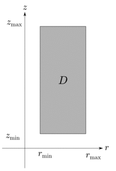
Consider a three-dimensional, axisymmetric body (of density  , Young's modulus
  , and Poisson's ratio
  ), occupying the region
  whose boundary is
  . Using cylindrical coordinates
  , the equations of linear elasticity can be written as
![\[
\nabla^* \cdot \bm{\tau}^* + \rho \mathbf{F}^* = \rho\frac{\partial^2\mathbf{u}^*}
{\partial {t^*}^2},
\]](form_6.png)
where  ,
,  is the stress tensor,
  is the body force and
  is the displacement field.
Note that, despite the fact that none of the above physical quantities depend on the azimuthal angle  , each can have a non-zero component. Also note that variables written with a superscript asterisk are dimensional, and their non-dimensional counterparts will be written without an asterisk. (The coordinate is, by definition, non-dimensional, so it will always be written without an asterisk.)
A boundary traction  and boundary displacement
  are imposed along the boundaries
  and
and  respectively, where
  so that
![\[
\mathbf{u}^* = \hat{\mathbf{u}}^*\text{ on }\partial D_\mathrm{d},
\qquad
\bm{\tau}^*\cdot\mathbf{n} = \hat{\bm{\tau}}^*\text{ on }\partial
D_\mathrm{n},
\]](form_17.png)
where  is the outer unit normal vector.
The constitutive equations relating the stresses to the displacements are
![\[
\bm{\tau}^* =
\frac{E}{1+\nu}\left(\frac{\nu}{1-2\nu}\left(\nabla^*\cdot\mathbf{u}^*\right)
\mathbf{I} + \frac{1}{2}\left(\nabla^*\mathbf{u}^* +
\left(\nabla^*\mathbf{u}^*\right)^\mathrm{T}\right)\right),
\]](form_19.png)
where  is the identity tensor and superscript
  denotes the transpose. In cylindrical coordinates, the matrix representation of the tensor
  is
is
![\[
\nabla^*\mathbf{u}^* =
\begin{pmatrix}
\dfrac{\strut \partial u_r^*}{\strut \partial r^*} &
-\dfrac{\strut u_\theta^*}{\strut r^*} & \dfrac{\strut \partial
u_r^*}{\strut \partial z^*}\\
\dfrac{\strut \partial u_\theta^*}{\strut \partial r^*} &
\dfrac{\strut u_r^*}{\strut r^*} & \dfrac{\strut \partial
u_\theta^*}{\strut \partial z^*}\\
\dfrac{\strut \partial u_z^*}{\strut \partial r^*} & 0
& \dfrac{\strut \partial u_z^*}{\strut \partial z^*}
\end{pmatrix}
\]](form_23.png)
and  is equal to the trace of this matrix.
We non-dimensionalise the equations, using a problem specific reference length,  , and a timescale
  , and use Young's modulus to non-dimensionalise the body force and the stress tensor:
![\[
\bm{\tau}^* = E \bm{\tau}, \qquad
r^* = \mathcal{L}r, \qquad
z^* = \mathcal{L}z
\]](form_27.png)
![\[
\mathbf{u}^* = \mathcal{L} \mathbf{u} \qquad
\mathbf{F}^* = \frac{E}{\rho \mathcal{L}}\mathbf{F},
\qquad
t^* = \mathcal{T}t.
\]](form_28.png)
The non-dimensional form of the axisymmetric linear elasticity equations is then given by
![\[
\nabla\cdot \bm{\tau} + \mathbf{F} = \Lambda^2\frac{\partial^2\mathbf{u}}
{\partial t^2},\qquad\qquad (1)
\]](form_29.png)
where  ,
,
![\[
\bm{\tau} =
\frac{1}{1+\nu}\left(\frac{\nu}{1-2\nu}\left(\nabla\cdot\mathbf{u}\right)
\mathbf{I} + \frac{1}{2}\left(\nabla\mathbf{u} +
\left(\nabla\mathbf{u}\right)^\mathrm{T}\right)\right),\qquad\qquad
(2)
\]](form_31.png)
and the non-dimensional parameter
![\[
\Lambda = \frac{\mathcal{L}}{\mathcal{T}}\sqrt{\frac{\rho}{E}}
\]](form_32.png)
is the ratio of the elastic body's intrinsic timescale,  , to the problem-specific timescale, , that we use for time-dependent problems. The boundary conditions are
![\[
\mathbf{u} = \hat{\mathbf{u}}\text{ on } \partial D_\mathrm{d}\qquad
\bm{\tau}\cdot\mathbf{n} = \hat{\bm{\tau}}\text{ on } \partial D_\mathrm{n}.
\]](form_34.png)
We must also specify initial conditions:
![\[
\left.\mathbf{u}\right|_{t=t_0} = \mathbf{u}^0,\qquad
\left.\frac{\partial\mathbf{u}}{\partial t}\right|_{t=t_0} =
\mathbf{v}^0.\qquad\qquad (3)
\]](form_35.png)
Implementation
Within oomph-lib, the non-dimensional version of the axisymmetric linear elasticity equations (1) combined with the constitutive equations (2) are implemented in the AxisymmetricLinearElasticityEquations class. This class implements the equations in a way which is general with respect to the specific element geometry. To obtain a fully functioning element class, we must combine the equations class with a specific geometric element class, as discussed in the (Not-So-)Quick Guide. For example, we will combine the AxisymmetricLinearElasticityEquations class with QElement<2,3> elements, which are 9-node quadrilateral elements, in our example problem. As usual, the mapping between local and global (Eulerian) coordinates within an element is given by
![\[
x_i = \sum_{j=1}^{N^{(E)}} X_{ij}^{(E)}\psi_j,\qquad i = 1,2,
\]](form_36.png)
where  ;
;  is the number of nodes in the element.
  is the
  -th global (Eulerian) coordinate of the
  -th node in the element and the
  are the element's shape functions, which are specific to each type of geometric element.
We store the three components of the displacement vector as nodal data in the order  and use the shape functions to interpolate the displacements as
![\[
u_i = \sum_{j=1}^{N^{(E)}}U_{ij}^{(E)}\psi_{ij},\qquad i = 1,\dotsc,3,
\]](form_44.png)
where  is the -th displacement component at the
  -th node in the element, i.e.,
 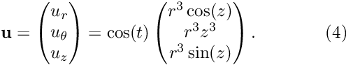 .
.
The solution of time dependent problems requires the specification of a TimeStepper that is capable of approximating second time derivatives. In the example problem below we use the Newmark timestepper.
The test problem
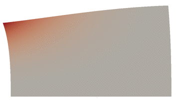
As a test problem we consider forced oscillations of the circular cylinder shown in the sketch below:
It is difficult to find non-trivial exact solutions of the governing equations (1), (2), so we manufacture a time-harmonic solution:
![\[
\mathbf{u} =
\begin{pmatrix}
u_r\\
u_\theta\\
u_z
\end{pmatrix} =
\cos(t)
\begin{pmatrix}
r^3\cos(z)\\
r^3z^3\\
r^3\sin(z)
\end{pmatrix}.\qquad\qquad (4)
\]](form_48.png)
This is an exact solution if we set the body force to
![\[
\mathbf{F} =
\cos(t)
\begin{pmatrix}
-r\cos(z)\left\{\left(8+3r\right)\lambda +
\left(16 - r\left(r-3\right)\right)\mu + r^2\Lambda^2\right\}\\
-r\left\{8z^3\mu + r^2\left(z^3\Lambda^2 + 6\mu z\right)\right\}\\
r\sin(z)\left\{- 9\mu + 4r\left(\lambda + \mu\right) +
r^2\left(\lambda + 2\mu -
\Lambda^2\right)\right\}
\end{pmatrix},\qquad\qquad (5)
\]](form_49.png)
where  and
and  are the nondimensional Lamé parameters. We impose the displacement along the boundaries
  according to (4), and impose the traction
![\[
\hat{\bm{\tau}}_3 = \bm{\tau}(r_\mathrm{min},z,t) =
\cos(\omega t)
\begin{pmatrix}
-\cos(z)r_\mathrm{min}^2\left(6\mu +
\lambda\left(4+r_\mathrm{min}\right)\right)\\
-2\mu r_\mathrm{min}^2z^3\\
-\mu r_\mathrm{min}^2\sin(z)\left(3-r_\mathrm{min}\right)
\end{pmatrix},\qquad\qquad (6)
\]](form_53.png)
along the boundary  .
.
The problem we are solving then consists of equations (1), (2) along with the body force, (5) and boundary traction (6). The initial conditions for the problem are the exact displacement, velocity (and acceleration; see below) according to the solution (4).
Results
The animation below shows the time dependent deformation of the cylinder in the  -
-  plane, while the colour contours indicate the azimuthal displacement component. The animation is for
 ![$ t \in [0,2\pi] $](form_57.png) , since the time scale is nondimensionalised on the reciprocal of the angular frequency of the oscillations.
, since the time scale is nondimensionalised on the reciprocal of the angular frequency of the oscillations.
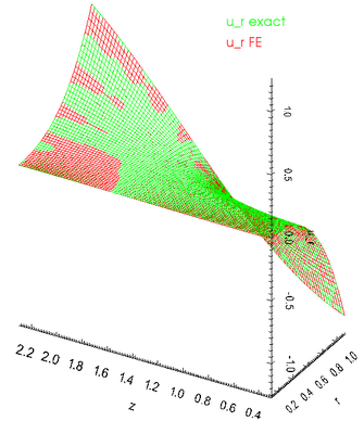
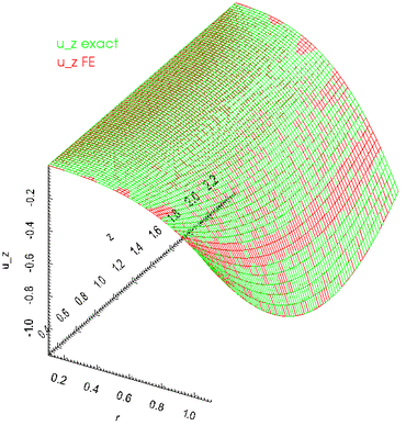
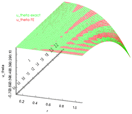
The next three figures show plots of the radial, axial and azimuthal displacements as functions of  at
at  . Note the excellent agreement between the numerical and exact solutions.
Global parameters and functions
As usual, we define all non-dimensional parameters in a namespace. In this namespace, we also define the body force, the traction to be applied on the boundary  , and the exact solution. Note that, consistent with the enumeration of the unknowns, discussed above, the order of the components in the functions that specify the body force and the surface traction is
  .
.
In addition, the namespace includes the necessary machinery for providing the time dependent equations with their initial data from the exact solution. There are 9 functions, one for each of the components of displacement, velocity and acceleration, and a helper function. For brevity, we list only one of these functions; the others are similar.
The driver code
We start by creating a DocInfo object that will be used to output the solution, and then build the problem.
Next we set up a timestepper and assign the initial conditions.
We calculate the number of timesteps to perform - if we are validating, just do small number of timesteps; otherwise do a full period the time-harmonic oscillation.
Finally we perform a time dependent simulation.
The problem class
The problem class is very simple, and similarly to other problems with Neumann conditions, there are separate meshes for the "bulk" elements and the "face" elements that apply the traction boundary conditions. The function assign_traction_elements() attaches the traction elements to the appropriate bulk elements.
The problem constructor
The problem constructor creates the mesh objects (which in turn create the elements), pins the appropriate boundary nodes and assigns the boundary conditions according to the functions defined in the Global_Parameters namespace.
Then the physical parameters are set for each element in the bulk mesh.
We then loop over the traction elements and set the applied traction.
Finally, we add the two meshes as sub-meshes, build a global mesh from these and assign the equation numbers.
The traction elements
We create the face elements that apply the traction to the boundary .
Initial data
The time integration in this problem is performed using the Newmark scheme which, in addition to the standard initial conditions (3), requires an initial value for the acceleration. Since we will be solving a test case in which the exact solution is known, we can use the exact solution to provide the complete set of initial data required. For the details of the Newmark scheme, see the tutorial on the linear wave equation.
If we're doing an impulsive start, set the displacement, velocity and acceleration to zero, and fill in the time history to be consistent with this.
If we are not doing an impulsive start, we must provide the timestepper with time history values for the displacement, velocity and acceleration. Each component of the these vectors is represented by a function pointer, and in this case, the function pointers return values based on the exact solution.
Then we loop over all nodes in the bulk mesh and set the initial data values from the exact solution.
Post-processing
This member function documents the computed solution to file and calculates the error between the computed solution and the exact solution.
Comments
- Given that we non-dimensionalised all stresses on Young's modulus it seems odd that we provide the option to specify a non-dimensional Young's modulus via the member function
AxisymmetricLinearElasticity::youngs_modulus_pt(). The explanation for this is that this function specifies the ratio of the material's actual Young's modulus to the Young's modulus used in the non-dimensionalisation of the equations. The capability to specify such ratios is important in problems where the elastic body is made of multiple materials with different constitutive properties. If the body is made of a single, homogeneous material, the specification of the non-dimensional Young's modulus is not required – it defaults to 1.0.
Exercises
- Try setting the boolean flag
impulsive_starttotruein theAxisymmetricLinearElasticityProblem::set_initial_conditionsfunction and compare the system's evolution to that obtained when a "smooth" start from the exact solution is performed. - Omit the specification of the Young's modulus and verify that the default value gives the same solution.
- Confirm that the assignment of the history values for the Newmark timestepper in
AxisymmetricLinearElasticityProblem::set_initial_conditionssets the correct initial values for the displacement, velocity and acceleration. (Hint: the relevant code is already contained in the driver code, but was omitted in the code listings shown above.)
Source files for this tutorial
- The source files for this tutorial are located in the directory:
demo_drivers/axisym_linear_elasticity/cylinder/
- The driver code is:
demo_drivers/axisym_linear_elasticity/cylinder/cylinder.cc
PDF file
A pdf version of this document is available. \