This is our first Navier-Stokes example problem. We discuss the non-dimensionalisation of the equations and their implementation in oomph-lib, and demonstrate the solution of the 2D driven cavity problem.

The Navier-Stokes equations

In dimensional form the 2D [3D] Navier-Stokes equations (in cartesian coordinates $x_i^*; \ i=1,2 [,3]$ ) are given by the momentum equations

$\rho\left(\frac{\partial u_i^*}{\partial t^*} + u_j^*\frac{\partial u_i^*}{\partial x_j^*}\right) = - \frac{\partial p^*}{\partial x_i^*} + B_i^*(x_j^*,t^*) + \rho \, G^*_i + \frac{\partial }{\partial x_j^*} \left[ \mu\left( \frac{\partial u_i^*}{\partial x_j^*} + \frac{\partial u_j^*}{\partial x_i^*} \right) \right],$

and the continuity equation

$\frac{\partial u_i^*}{\partial x_i^*} = Q^*,$

where we have used index notation and the summation convention.

Here, the velocity components are denoted by , the pressure by , and time by , and we have split the body force into two components: A constant vector $\rho \, G_i^*$ which typically represents gravitational forces; and a variable body force, . is a volumetric source term for the continuity equation and is typically equal to zero.

We non-dimensionalise the equations, using problem-specific reference quantities for the velocity, ${\cal U},$ length, ${\cal L},$ and time, ${\cal T},$ and scale the constant body force vector on the gravitational acceleration, so that

$u_i^* = {\cal U} \, u_i, \qquad x_i^* = {\cal L}\, x_i, \qquad t^* = {\cal T}\, t, \qquad G_i^* = g \, G_i,$

$p^* = \frac{\mu_{ref} {\cal U}}{{\cal L}} \, p, \qquad B_i^* = \frac{{\cal U}\mu_{ref}}{{\cal L}^2} \, B_i, \qquad Q^* = \frac{{\cal U}}{{\cal L}}\, Q, \qquad$

where we note that the pressure and the variable body force have been non-dimensionalised on the viscous scale. $\mu_{ref}$ and $\rho_{ref}$ (used below) are reference values for the fluid viscosity and density, respectively. In single-fluid problems, they are identical to the viscosity $\mu$ and density $\rho$ of the (one and only) fluid in the problem.

The non-dimensional form of the Navier-Stokes equations is then given by

$R_\rho Re \left( St \frac{\partial u_i}{\partial t} + u_j \frac{\partial u_i}{\partial x_j} \right) = - \frac{\partial p}{\partial x_i} + B_i(x_j,t) + R_\rho \frac{Re}{Fr} G_i + \frac{\partial }{\partial x_j} \left[ R_\mu \left( \frac{\partial u_i}{\partial x_j} + \frac{\partial u_j}{\partial x_i} \right) \right],$

and

$\frac{\partial u_i}{\partial x_i} = Q,$

where the dimensionless parameters

$Re = \frac{{\cal U}{\cal L}\rho_{ref}}{\mu_{ref}}, \qquad St = \frac{{\cal L}}{{\cal U}{\cal T}}, \qquad Fr = \frac{{\cal U}^2}{g{\cal L}},$

are the Reynolds number, Strouhal number and Froude number respectively. $R_\rho=\rho/\rho_{ref}$ and $R_\mu =\mu/\mu_{ref}$ represent the ratios of the fluid's density and its dynamic viscosity, relative to the density and viscosity values used to form the non-dimensional parameters (By default, $R_\rho = R_\mu = 1$ ; other values tend to be used in problems involving multiple fluids).

The above equations are typically augmented by Dirichlet boundary conditions for (some of) the velocity components. On boundaries where no velocity boundary conditions are applied, the flow satisfies the "traction free" natural boundary condition $t_i = -p \, n_i + R_\mu (\partial u_i/\partial x_j + \partial u_j/\partial x_i ) \, n_j = 0.$ (We refer to another example for an illustration of how to apply traction boundary conditions for the Navier-Stokes equations.)

If the velocity is prescribed along the entire domain boundary, the fluid pressure is only determined up to an arbitrary constant. This indeterminacy may be overcome by prescribing the value of the pressure at a single point in the domain (see exercise).

Implementation

The elements

oomph-lib provides two LBB-stable isoparametric Navier-Stokes elements that are based on the QElement<DIM,3> family of geometric finite elements. They are nine-node quadrilateral (for DIM=2), and 27-node brick (for DIM=3) elements in which the mapping between local and global (Eulerian) coordinates is given by

$x_i = \sum_{j=1}^{N^{(E)}} X^{(E)}_{ij} \, \psi_j, \qquad i=1,2\quad [\mbox{and }3].$

Here $N^{(E)} = 3^{DIM}$ is the number of nodes in the element, $X^{(E)}_{ij}$ is the -th global (Eulerian) coordinate of the -th Node in the element, and the $\psi_j$ are the element's geometric shape functions, defined in the QElement<DIM,3> class.

In both elements the velocity components [and ] are stored as nodal values and the geometric shape functions are used to interpolate the velocities inside the element,

$u_i = \sum_{j=1}^{N^{(E)}} U^{(E)}_{ij} \, \psi_j, \qquad i=1,2\quad [\mbox{and }3],$

where $U^{(E)}_{ij}$ is the -th velocity component at -th Node in the element. Nodal values of the velocity components are accessible via the access function

NavierStokesEquations<DIM>::u(i,j)

which returns the i-th velocity component stored at the element's j-th Node.

The two elements differ in the way in which the pressure is represented:

Crouzeix-Raviart elements

In oomph-lib's QCrouzeixRaviartElements the pressure is represented by,

$p = P_0^{(E)} + P_1^{(E)} \, s_1 + P_2^{(E)} \, s_2 \quad \left[+ P_3^{(E)} \, s_3\right],$

where the $s_i \in [-1,1]$ are the element's local coordinates. This provides a discontinuous, piecewise bi-[tri-]linear representation of the pressure in terms of 3 [4] pressure degrees of freedom per element. Crouzeix-Raviart elements ensure that the continuity equation is satisfied within each element.

The pressure degrees of freedom are local to the element and are stored in the element's internal Data. They are accessible via the member function

QCrouzeixRaviartElement<DIM>::p(j)

which returns the value of the j-th pressure degree of freedom in this element.

Each Node in a 2D [3D] Crouzeix-Raviart element stores 2 [3] nodal values, representing the two [three] velocity components at that Node.

Taylor-Hood elements

In oomph-lib's QTaylorHoodElements the pressure is represented by a globally-continuous, piecewise bi-[tri-]linear interpolation between the pressure values $P_j^{(E)}$ that are stored at the elements' $N_p^{(E)} = 2^{DIM}$ corner/vertex nodes,

$p = \sum_{j=1}^{N_p^{(E)}} P_j^{(E)} \, \psi_j^{(p)},$

where the $\psi_j^{(p)}$ are the bi-[tri-]linear pressure shape functions.

The first 2 [3] values of each Node in a 2D [3D] Taylor-Hood element store the two [three] velocity components at that Node. The corner [vertex] nodes store an additional value which represents the pressure at that Node. The access function

QTaylorHoodElement<DIM>::p(j)

returns the nodal pressure value at the element's j-th corner [vertex] Node.

In sufficiently fine meshes, Taylor-Hood elements generate a much smaller number of pressure degrees of freedom than the corresponding Crouzeix-Raviart elements. However, Taylor-Hood elements do not conserve mass locally.

Non-dimensional parameters and their default values

The Reynolds number, Strouhal number, inverse-Froude number, density ratio and viscosity ratio are assumed to be constant within each element. Their values are accessed via pointers which are accessible via the member functions re_pt() for re_st_pt() for $Re \ St,$ re_invfr_pt() for density_ratio_pt() for $R_\rho$ and viscosity_ratio_pt() for $R_\mu$ .

By default the pointers point to default values (implemented as static member data in the NavierStokesEquations class), therefore they only need to be over-written if the default values are not appropriate. The default values are:

Default Reynolds number:
$Re = 0 \mbox{\ \ \ \ (Stokes flow)}$
Default Womersley number (product of Reynolds and Strouhal number):
$Re St = 0 \mbox{\ \ \ \ (steady flow)}$
Default product of Reynolds and inverse Froude number (a measure of gravity on the viscous scale)
$Re/Fr = 0 \mbox{\ \ \ \ (no gravity)}$
Default viscosity ratio:
$R_\mu = 1 \mbox{\ \ \ \ (viscosity = viscosity used in the definition of $Re$)}$
Default density ratio:
$R_\rho = 1 \mbox{\ \ \ \ (density = density used in the definition of $Re$)}$

We use the same approach for the specification of the body force vector , accessible via the function g_pt (), the variable body force , accessible via the function pointer body_force_fct_pt(), and the volumetric source function , accessible via the function pointer source_fct_pt(time,x). By default the (function) pointers are set such that

Default gravity vector:
$G_i = 0 \mbox{\ \ \ \ (no gravity)}$
Default body force function:
$B_i(x_j,t) = 0 \mbox{\ \ \ \ (no body force)}$
Default volumetric source function
$Q(x_j,t) = 0 \mbox{\ \ \ \ (flow is divergence free)}$

The example problem

We will illustrate the solution of the steady 2D Navier-Stokes equations using the well-known example of the driven cavity.

The 2D steady driven-cavity problem in a square domain. Solve

$Re\phantom{i}u_j\frac{\partial u_i}{\partial x_j} = - \frac{\partial p}{\partial x_i} + \frac{\partial }{\partial x_j} \left( \frac{\partial u_i}{\partial x_j} + \frac{\partial u_j}{\partial x_i} \right), \ \ \ \ \ \ \ \ \ \ (1)$

and

$\frac{\partial u_i}{\partial x_i} = 0,$

in the square domain

, subject to the Dirichlet boundary conditions:

$\left. \mathbf{u}\right|_{\partial D}=(0,0), \ \ \ \ \ \ \ \ \ \ (2)$

on the right, top and left boundaries and

$\left. \mathbf{u}\right|_{\partial D}=(1,0), \ \ \ \ \ \ \ \ \ \ (3)$

on the bottom boundary,

Results

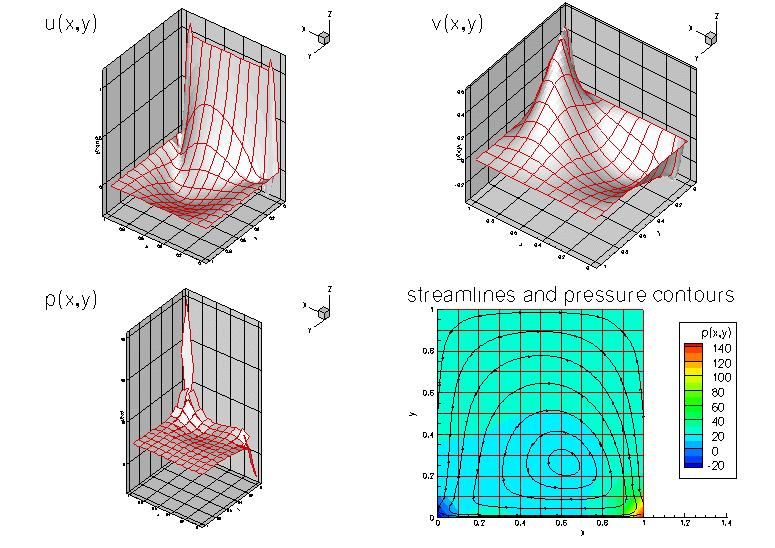
Crouzeix-Raviart elements

The figure below shows "carpet plots" of the velocity and pressure fields as well as a contour plot of the pressure distribution with superimposed streamlines. The velocity vanishes along the entire domain boundary, apart from the bottom boundary where the moving "lid" imposes a unit tangential velocity which drives a large vortex, centred at 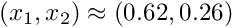$(x_1,x_2) \approx (0.62,0.26)$ . The discontinuity in the velocity boundary conditions creates pressure singularities at and . The rapidly varying pressure in the vicinity of these points clearly shows the discontinuous pressure interpolation employed by the Crouzeix-Raviart elements.

Plot of the velocity and pressure fields for Re=100 computed with Crouzeix-Raviart (Q2P-1) elements.

Taylor-Hood elements

The next figure shows the corresponding results obtained from a computation with QTaylorHoodElements. The pressure plot illustrates how the interpolation between the corner nodes creates a globally continuous representation of the pressure.

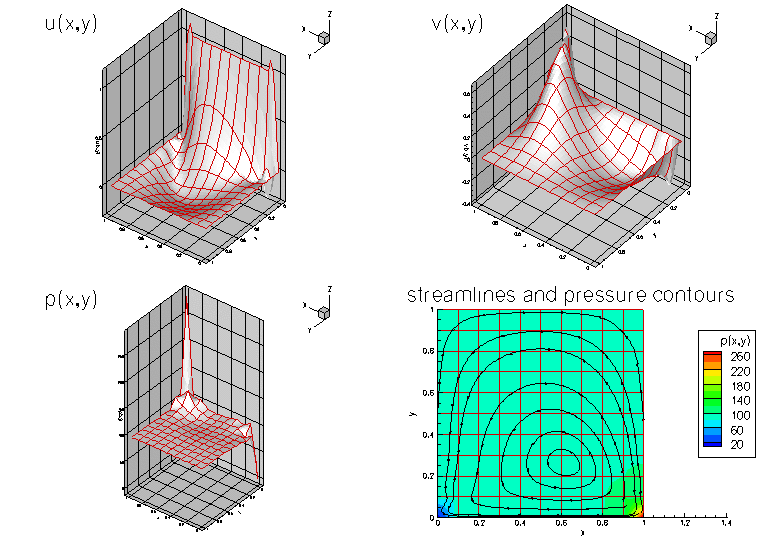
Plot of the velocity and pressure fields for Re=100 computed with Taylor-Hood (Q2Q1) elements.

Note that in both simulations, the flow field is clearly under-resolved near the ends of the "lid". In another example we will demonstrate the use of spatial adaptivity to obtain much better solutions for this problem.

Global parameters and functions

The Reynolds number is the only non-dimensional parameter needed in this problem. As usual, we define it in a namespace:

//==start_of_namespace==============================
/// Namespace for physical parameters
//==================================================
namespace Global_Physical_Variables
{
 
 /// Reynolds number
 double Re=100;
 
} // end_of_namespace

The driver code

We start by creating a DocInfo object to store the output directory and the label for the output files.

//==start_of_main======================================================
/// Driver for RectangularDrivenCavity test problem -- test drive
/// with two different types of element.
//=====================================================================
int main()
{
 
 // Set up doc info
 // ---------------
 
 // Label for output
 DocInfo doc_info;
 
 // Set output directory
 doc_info.set_directory("RESLT");
 
 // Step number
 doc_info.number()=0;

We build the problem using QCrouzeixRaviartElements, solve using the Problem::newton_solve() function, and document the result before incrementing the label for the output files.

 // Doing QCrouzeixRaviartElements
 {
  
  // Build the problem with QCrouzeixRaviartElements
  RectangularDrivenCavityProblem<QCrouzeixRaviartElement<2> > problem;
  cout << "Doing QCrouzeixRaviartElement<2>" << std::endl;
  
  // Solve the problem
  problem.newton_solve();
  
  // Outpt the solution
  problem.doc_solution(doc_info);
 
  // Step number
  doc_info.number()++;
 
 } // end of QCrouzeixRaviartElements

Finally, we repeat the process with QTaylorHoodElements.

 // Doing QTaylorHoodElements
 {
  
  // Build the problem with QTaylorHoodElements
  RectangularDrivenCavityProblem<QTaylorHoodElement<2> > problem;
  cout << "Doing QTaylorHoodElement<2>" << std::endl;
  
  // Solve the problem
  problem.newton_solve();
  
  // Outpt the solution
  problem.doc_solution(doc_info);
 
  // Step number
  doc_info.number()++;
 
 } // end of QTaylorHoodElements
 
 
} // end_of_main

The problem class

The Problem class for our steady Navier-Stokes problem is very similar to those used for the steady scalar problems (Poisson and advection-diffusion) that we considered in previous examples. We provide a helper function fix_pressure(...) which pins a pressure value in a specified element and assigns a specific value.

//==start_of_problem_class============================================
/// Driven cavity problem in rectangular domain
//====================================================================
template<class ELEMENT>
class RectangularDrivenCavityProblem : public Problem
{
 
public:
 
 
 /// Constructor
 RectangularDrivenCavityProblem();
 
 /// Destructor (empty)
 ~RectangularDrivenCavityProblem(){}
 
 /// Fix pressure in element e at pressure dof pdof and set to pvalue
 void fix_pressure(const unsigned &e, const unsigned &pdof, 
                   const double &pvalue)
  {
   //Cast to full element type and fix the pressure at that element
   dynamic_cast<ELEMENT*>(mesh_pt()->element_pt(e))->
                          fix_pressure(pdof,pvalue);
  } // end of fix_pressure

No actions are performed after the solution is found, since the solution is documented in main. However, before solving, the boundary conditions must be set.

 /// Update the after solve (empty)
 void actions_after_newton_solve(){}
 
 
 /// Update the problem specs before solve. 
 /// Re-set velocity boundary conditions just to be on the safe side...
 void actions_before_newton_solve()
 {
  // Setup tangential flow along boundary 0:
  unsigned ibound=0; 
  unsigned num_nod= mesh_pt()->nboundary_node(ibound);
  for (unsigned inod=0;inod<num_nod;inod++)
   {
    // Tangential flow
    unsigned i=0;
    mesh_pt()->boundary_node_pt(ibound,inod)->set_value(i,1.0);
    // No penetration
    i=1;
    mesh_pt()->boundary_node_pt(ibound,inod)->set_value(i,0.0);
   }
  
  // Overwrite with no flow along the other boundaries
  unsigned num_bound = mesh_pt()->nboundary();
  for(unsigned ibound=1;ibound<num_bound;ibound++)
   {
    unsigned num_nod= mesh_pt()->nboundary_node(ibound);
    for (unsigned inod=0;inod<num_nod;inod++)
     {
      for (unsigned i=0;i<2;i++)
       {
        mesh_pt()->boundary_node_pt(ibound,inod)->set_value(i,0.0);
       }
     }
   }
 } // end_of_actions_before_newton_solve

Finally, we provide an access function to the specific mesh and define the post-processing function doc_solution(...).

 // Access function for the specific mesh
 SimpleRectangularQuadMesh<ELEMENT>* mesh_pt() 
  {
   // Upcast from pointer to the Mesh base class to the specific 
   // element type that we're using here.
   return dynamic_cast<SimpleRectangularQuadMesh<ELEMENT>*>(
    Problem::mesh_pt());
  }
 
 
 /// Doc the solution
 void doc_solution(DocInfo& doc_info);
 
}; // end_of_problem_class

The problem constructor

Since this is a steady problem, the constructor is quite simple. We begin by building the mesh and pin the velocities on the boundaries.

//==start_of_constructor==================================================
/// Constructor for RectangularDrivenCavity problem 
//========================================================================
template<class ELEMENT>
RectangularDrivenCavityProblem<ELEMENT>::RectangularDrivenCavityProblem()
{ 
 
 // Setup mesh
 
 // # of elements in x-direction
 unsigned n_x=10;
 
 // # of elements in y-direction
 unsigned n_y=10;
 
 // Domain length in x-direction
 double l_x=1.0;
 
 // Domain length in y-direction
 double l_y=1.0;
 
 // Build and assign mesh
 Problem::mesh_pt() = new SimpleRectangularQuadMesh<ELEMENT>(n_x,n_y,l_x,l_y);
 
 // Set the boundary conditions for this problem: All nodes are
 // free by default -- just pin the ones that have Dirichlet conditions
 // here. 
 unsigned num_bound = mesh_pt()->nboundary();
 for(unsigned ibound=0;ibound<num_bound;ibound++)
  {
   unsigned num_nod= mesh_pt()->nboundary_node(ibound);
   for (unsigned inod=0;inod<num_nod;inod++)
    {
     // Loop over values (u and v velocities)
     for (unsigned i=0;i<2;i++)
      {
       mesh_pt()->boundary_node_pt(ibound,inod)->pin(i); 
      }
    }
  } // end loop over boundaries

Next we pass a pointer to the Reynolds number (stored in Global_Physical_Variables::Re) to all elements.

 // Complete the build of all elements so they are fully functional
 
 //Find number of elements in mesh
 unsigned n_element = mesh_pt()->nelement();
 
 // Loop over the elements to set up element-specific 
 // things that cannot be handled by constructor
 for(unsigned e=0;e<n_element;e++)
  {
   // Upcast from GeneralisedElement to the present element
   ELEMENT* el_pt = dynamic_cast<ELEMENT*>(mesh_pt()->element_pt(e));
 
   //Set the Reynolds number
   el_pt->re_pt() = &Global_Physical_Variables::Re;
  } // end loop over elements

Since Dirichlet conditions are applied to both velocity components on all boundaries, the pressure is only determined up to an arbitrary constant. We use the fix_pressure(...) function to pin the first pressure value in the first element and set its value to zero.

// Now set the first pressure value in element 0 to 0.0

fix_pressure(0,0,0.0);

Finally, the equation numbering scheme is set up, using the function assign_eqn_numbers().

 // Setup equation numbering scheme
 cout <<"Number of equations: " << assign_eqn_numbers() << std::endl; 
} // end_of_constructor

Post-processing

As expected, this member function documents the computed solution.

//==start_of_doc_solution=================================================
/// Doc the solution
//========================================================================
template<class ELEMENT>
void RectangularDrivenCavityProblem<ELEMENT>::doc_solution(DocInfo& doc_info)
{ 
 ofstream some_file;
 char filename[100];
 
 // Number of plot points
 unsigned npts;
 npts=5; 
 
 // Output solution 
 sprintf(filename,"%s/soln%i.dat",doc_info.directory().c_str(),
         doc_info.number());
 some_file.open(filename);
 mesh_pt()->output(some_file,npts);
 some_file.close();
} // end_of_doc_solution

Comments and Exercises

The stress-divergence form

As discussed in the introduction, by default oomph-lib's Navier-Stokes elements use the stress-divergence form of the momentum equations,

$R_\rho Re \left( St \frac{\partial u_i}{\partial t} + u_j \frac{\partial u_i}{\partial x_j} \right) = - \frac{\partial p}{\partial x_i} + B_i(x_j) + R_\rho \frac{Re}{Fr} G_i + \frac{\partial }{\partial x_j} \left[ R_\mu \left( \frac{\partial u_i}{\partial x_j} + \frac{\partial u_j}{\partial x_i} \right) \right],$

as this form is required in problems with free surfaces or problems in which traction boundary conditions are applied.

If the flow is divergence free ( $Q = 0 \Longrightarrow \partial u_i/\partial x_i =0$ ), the viscous term may be simplified to

assuming that the viscosity ratio $R_\mu$ remains constant

This simpler form of the equations can be used to solve problems that do not incorporate traction boundaries or free surfaces. We illustrate the use of these equations in another example.

Exercises

Compare the pressure distributions obtained with Taylor-Hood elements to that computed with Crouzeix-Raviart elements. Why do they differ? [Hint: Consider how the pressure is represented in the two elements.]
Confirm that the velocities stored at boundary nodes must be pinned. Investigate what happens if you do not apply any velocity boundary conditions [Hint: You should still be able to
compute a solution – what does this solution represent?]
Investigate what happens when no pressure value is fixed.

Source files for this tutorial

The source files for this tutorial are located in the directory: demo_drivers/navier_stokes/driven_cavity/
The driver code is: demo_drivers/navier_stokes/driven_cavity/driven_cavity.cc

PDF file

A pdf version of this document is available.