In this document we discuss the solution of time-harmonic acoustic fluid-structure interaction problems. We start by reviewing the relevant theory and then present the solution of a simple model problem – the sound radiation from an oscillating circular cylinder that is coated with a compressible elastic layer.

This problem combines the problems discussed in the tutorials illustrating

the solution of the time-harmonic equations of linear elasticity

and

the Helmholtz equation.

Theory: Time-harmonic acoustic fluid-structure interaction problems

The figure below shows a sketch of a representative model problem: a circular cylinder is immersed in an inviscid compressible fluid and performs a prescribed two-dimensional harmonic oscillation of radian frequency $\omega$ . The cylinder is coated with a compressible elastic layer. We wish to compute the displacement field in the elastic coating (assumed to be described by the equations of time-harmonic linear elasticity) and the pressure distribution in the fluid (governed by the Helmholtz equation). The two sets of equations interact at the interface between fluid and solid: the fluid pressure exerts a traction onto the elastic layer, while the motion of the elastic layer drives the fluid motion via the non-penetration condition.

Sketch of the model problem: Forced oscillations of a circular cylinder (black) deform an elastic coating layer (pink) which is surrounded by a compressible fluid.

The fluid model: the Helmholtz equation

We describe the behaviour of the fluid in terms of the displacement field, , of the fluid particles. As usual we employ index notation and the summation convention, and use asterisks to distinguish dimensional quantities from their non-dimensional equivalents. The fluid is inviscid and compressible, with a bulk modulus , such that the acoustic pressure is given by $P^* = - B \ \partial d_j^*/\partial x_j^*$ We assume that the fluid motion is irrotational and can be described by a displacement potential $\Phi^*$ , such that $d^*_j = \partial \Phi^*/\partial x_j^*.$ We consider steady-state time-harmonic oscillations and write the displacement potential and the pressure as $\Phi^*(x_j^*,t^*) = \mbox{Re} \{\phi^*(x_j^*) \exp(-{\rm i} \omega t^*)\}$ and $P^*(x_j^*,t^*) = \mbox{Re}\{p^*(x_j^*) \exp(-{\rm i} \omega t^*)\}$ , respectively, where $\mbox{Re}\{\ldots \}$ denotes the real part. For small disturbances, the linearised Euler equation reveals that the time-harmonic pressure is related to the displacement potential via $p^* = \rho_{\rm f} \omega^2 \phi^*$ where $\rho_{\rm f}$ is the ambient fluid density. We non-dimensionalise all lengths on a problem-specific lengthscale ${\cal L}$ (e.g. the outer radius of the coating layer) such that $x_j^* = {\cal L} x_j,\ d_j^* = {\cal L} d_j$ and $\phi^* = {\cal L}^2 \phi$ . The non-dimensional displacement potential $\phi$ is then governed by the Helmholtz equation

$\frac{\partial^2 \phi}{\partial x_j^{2}} + k^2 \phi = 0, \ \ \ \ \ \ \ \ \ \ \ \ \ \ \ \ \ \ \ \ \ \ (1)$

where the square of the non-dimensional wavenumber,

$k^2 = \frac{\rho_f (\omega {\cal L})^2}{B},$

represents the ratio of the typical inertial fluid pressure induced by the wall oscillation to the ‘stiffness’ of the fluid.

The solid model: the time harmonic equations of linear elasticity

We model the coating layer as a linearly elastic solid, described in terms of a displacement field , with stress tensor

$\tau_{ij}^* = E \left[ \frac{\nu}{(1+\nu)(1-2\nu)} \, \frac{\partial U_k^*}{\partial x_k^*} \, \delta_{ij} +\frac{1}{2(1+\nu)}\left( \frac{\partial U_i^*}{\partial x_j^*}+ \frac{\partial U_j^*}{\partial x_i^*} \right) \right],$

where and $\nu$ are the material's Young's modulus and Poisson's ratio, respectively. As before, we assume a time-harmonic solution with frequency $\omega$ so that $U_i^*(x_j^*,t^*) = {\rm Re} \{ u_i^*(x_j^*) \exp(-{\rm i}\omega t^*)\}$ , and we non-dimensionalise the displacements on ${\cal L}$ and the stress on Young's modulus, , so that $u_j^* = {\cal L} u_j$ and $\tau_{ij}^* = E \tau_{ij}$ . The deformation of the elastic coating is then governed by the time-harmonic Navier-Lame equations

$\frac{\partial \tau_{ij}}{\partial x_j} + \Omega^2 u_i = 0, \ \ \ \ \ \ \ \ \ \ \ \ \ \ \ \ \ \ \ \ \ \ (2)$

which depend (implicitly) on Poisson's ratio $\nu$ , and on the (square of the) non-dimensional wavenumber

$\Omega^2 = \frac{\rho_{\rm s} (\omega {\cal L})^2}{E},$

where $\rho_{\rm s}$ is the solid density. The parameter $\Omega^2$ represents the ratio of the typical inertial solid pressure induced by the wall oscillation to the stiffness of the elastic coating. We note that for a ‘light’ coating we have $\Omega \ll 1$ .

Boundary conditions

The inner surface of the elastic coating, $\partial D_{\rm s}$ , is subject to the prescribed displacement imposed by the oscillating cylinder. For instance, if the inner cylinder performs axisymmetric oscillations of non-dimensional amplitude $\epsilon$ , we have

$\mbox{\bf u} = \epsilon \, \mbox{\bf e}_r \mbox{\ \ \ \ \ on $\partial D_{\rm s}$}, \ \ \ \ \ \ \ \ \ \ \ \ \ \ \ \ \ \ \ \ \ \ (3)$

where $\mbox{\bf e}_r$ is the unit vector in the radial direction. The fluid-loaded surface of the elastic coating, $\partial D_{\rm f}$ , is subject to the fluid pressure. The non-dimensional traction exerted by the fluid onto the solid (on the solid stress scale) is therefore given by

$t_i^{\rm [solid]} = \tau_{ij}^{\rm [solid]} n_j = - \phi \ Q \ n_i \mbox{\ \ \ \ \ on $\partial D_{\rm f}$}, \ \ \ \ \ \ \ \ \ \ \ \ \ \ \ \ \ \ \ \ \ \ (4)$

where the are the components of the outer unit normal on the solid boundary $\partial D_{\rm f}$ and

$Q=\frac{\rho_{\rm f}({\cal L}\omega)^2}{E}$

is the final non-dimensional parameter in the problem. It represents the ratio of the typical inertial fluid pressure induced by the wall oscillation to the stiffness of the elastic coating. The parameter therefore provides a measure of the strength of the fluid-structure interaction (FSI) in the sense that for $Q \to 0$ the elastic coating does not ‘feel’ the presence of the fluid.

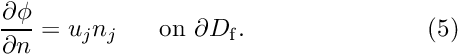The fluid is forced by the normal displacement of the solid. Imposing the non-penetration condition on $\partial D_{\rm f}$ yields a Neumann condition for the displacement potential,

$\frac{\partial \phi}{\partial n} = u_j n_j \mbox{\ \ \ \ \ on $\partial D_{\rm f}$}. \ \ \ \ \ \ \ \ \ \ \ \ \ \ \ \ \ \ \ \ \ \ (5)$

Finally, the displacement potential for the fluid must satisfy the Sommerfeld radiation condition

$\lim_{r \to \infty} \sqrt{r}\left( \frac{\partial \phi}{\partial r} - {\rm i} k \phi \right) = 0 \ \ \ \ \ \ \ \ \ \ \ \ \ \ \ \ \ \ \ \ \ \ (6)$

which ensures that the oscillating cylinder does not generate any incoming waves.

Implementation

The implementation of the coupled problem follows the usual procedure for multi-domain problems in oomph-lib. We discretise the constituent single-physics problems using the existing single-physics elements, here oomph-lib's

Helmholtz elements

and

time-harmonic linear elasticity elements

for the discretisation of the PDEs (1) and (2), respectively. The displacement boundary condition (3) on the inner surface of the elastic coating is imposed as usual by pinning the relevant degrees of freedom, exactly as in a single-physics solid mechanics problem. Similarly, the Sommerfeld radiation condition (6) on the outer boundary of the fluid domain can be imposed by any of the methods available for the solution of the single-physics Helmholtz equation, such as approximate/absorbing boundary conditions (ABCs) or a Dirichlet-to-Neumann mapping.

The boundary conditions (4) and (5) at the fluid-solid interface are traction boundary conditions for the solid, and Neumann boundary conditions for the Helmholtz equation, respectively. In a single-physics problem we would impose such boundary conditions by attaching suitable FaceElements to the appropriate boundaries of the "bulk" elements, as shown in the sketch below: TimeHarmonicLinearElasticityTractionElements could be used to impose a (given) traction, ${\bf t}_0$ , onto the solid; HelmholtzFluxElements could be used to impose a (given) normal derivative, , on the displacement potential. Both ${\bf t}_0$ and would usually be specified in a user-defined namespace and accessed via function pointers as indicated in the right half of the sketch.

Sketch illustrating the imposition of flux and traction boundary conditions in single-physics problems. The continuous problems are shown on the left; the discretised ones on the right.

In the coupled problem, illustrated in the left half of the next sketch, the traction acting on the solid becomes a function of the displacement potential via the boundary condition (4), while the normal derivative of the displacement potential is given in terms of the solid displacement via equation (5). Note that corresponding points on the FSI boundary $\partial D_{\rm f}$ are identified by matching values of the boundary coordinate $\zeta$ which is assumed to be consistent between the two domains.

The implementation of this interaction in the discretised problem is illustrated in the right half of the sketch: We replace the single-physics HelmholtzFluxElements by HelmholtzFluxFromNormalDisplacementBCElements, and the TimeHarmonicLinearElasticityTractionElements by TimeHarmonicLinElastLoadedByHelmholtzPressureBCElements. (Yes, we like to be verbose...). Both of these FaceElements are derived from the ElementWithExternalElement base class and can therefore store a pointer to an "external" element that provides the information required to impose the appropriate boundary condition. Thus, the HelmholtzFluxFromNormalDisplacementBCElements store pointers to the "adjacent" time-harmonic linear elasticity elements (from which they obtain the boundary displacement required for the imposition of (5)), while the TimeHarmonicLinElastLoadedByHelmholtzPressureBCElements store pointers to the "adjacent" Helmholtz elements that provide the value of the displacement potential required for the evaluation of (4).

Sketch illustrating the imposition of flux and traction boundary conditions in the coupled multi-physics problem. The continuous problems are shown on the left; the discretised ones on the right.

The identification of the "adjacent" bulk elements can be performed using the Multi_domain_functions::setup_bulk_elements_adjacent_to_face_mesh(...) helper function. We note that, as suggested by the sketch above, this function does not require to the two adjacent meshes to have a consistent discretisation – the identification of adjacent elements is based entirely on the (assumed to be consistent) boundary coordinate $\zeta$ in the two meshes. We refer to another tutorial for a discussion of how to set up (or change) the parametrisation of mesh boundaries by boundary coordinates.

Results

The animation below shows the deformation of the elastic coating if a non-axisymmetric displacement

$\mbox{\bf u} = \epsilon \, \mbox{\bf e}_r \cos (N\varphi) \mbox{\ \ \ \ \ on $\partial D_{\rm s}$}, \ \ \ \ \ \ \ \ \ \ \ \ \ \ \ \ \ \ \ \ \ \ (7)$

(for ) is imposed on the inner boundary of the coating $\partial D_{\rm s}$ .

Animation showing the time-harmonic oscillation of the elastic coating. (The pink region in the background shows the undeformed configuration.)

Here is a plot of the corresponding pressure field:

Plot of the displacement potential (a measure of the fluid pressure). The elevation in the carpet plot indicates the real part; the colour contours represent the imaginary part.

Finally, we provide some validation of the computational results by comparing the non-dimensional time-average radiated power

$\overline{\cal P} = \frac{1}{2} \oint\bigg[Im\bigg(\frac{\partial \phi}{\partial n}\bigg) \ Re(\phi) - Re\bigg(\frac{\partial \phi}{\partial n}\bigg) \ Im(\phi) \bigg] \ dS \ \ \ \ \ \ \ \ \ \ \ \ \ \ \ \ \ \ \ \ \ \ (8)$

against the analytical solution for axisymmetric forcing ( ) for the parameter values , $\Omega^2 = 0$ , $\nu =0.3$ and a non-dimensional coating thickness of see Heil, M., Kharrat, T., Cotterill, P.A. & Abrahams, I.D. (2012) Quasi-resonances in sound-insulating coatings. Journal of Sound and Vibration 331 4774-4784 for details. In the computations the integral in (8) is evaluated along the outer boundary of the computational domain.

Radiated power as function of the FSI parameter Q for an axisymmetrically oscillating coating. Markers: computed results; continuous line: analytical result.

The numerical solution

The global namespace

As usual we define the problem parameters in a namespace.

//=======start_namespace==========================================
/// Global variables
//================================================================
namespace Global_Parameters
{
 
 /// Square of wavenumber for the Helmholtz equation
 double K_squared=10.0;
 
 /// Radius of outer boundary of Helmholtz domain
 double Outer_radius=4.0; 
 
 /// FSI parameter
 double Q=0.0;
 
 /// Non-dim thickness of elastic coating
 double H_coating=0.3; 
 
 /// Poisson's ratio
 double Nu = 0.3;
 
 /// The elasticity tensor for the solid
 TimeHarmonicIsotropicElasticityTensor E(Nu);

We wish to perform parameter studies in which we vary the FSI parameter . To make this physically meaningful, we interpret $Q =(\rho_{\rm f}({\cal L}\omega)^2)/E$ as a measure of the stiffness of the elastic coating (so that an increase in corresponds to a reduction in the layer's elastic modulus ). In that case, the frequency parameter $\Omega^2 = (\rho_{\rm s} (\omega {\cal L})^2)/E$ in the time-harmonic linear elasticity equations becomes a dependent parameter and is given in terms of the density ratio $\rho_{\rm solid}/\rho_{\rm fluid}$ and by $\Omega^2 = (\rho_{\rm solid}/\rho_{\rm fluid}) Q$ . We therefore provide a helper function to update the dependent parameter following any change in the independent parameters.

  
 /// Density ratio: solid to fluid
 double Density_ratio=0.0;
 
 /// Non-dim square of frequency for solid -- dependent variable!
 double Omega_sq=0.0;
 
 /// Function to update dependent parameter values
 void update_parameter_values()
 {
  Omega_sq=Density_ratio*Q;
 }

We force the system by imposing a prescribed displacement on the inner surface of the elastic coating and allow this to vary in the azimuthal direction with wavenumber :

 
 /// Azimuthal wavenumber for imposed displacement of coating
 /// on inner boundary 
 unsigned N=0; 
 
 /// Displacement field on inner boundary of solid
 void solid_boundary_displacement(const Vector<double>& x,
                                  Vector<std::complex<double> >& u)
 {
  Vector<double> normal(2);
  double norm=sqrt(x[0]*x[0]+x[1]*x[1]);
  double phi=atan2(x[1],x[0]);
  normal[0]=x[0]/norm;
  normal[1]=x[1]/norm;
 
  u[0]=complex<double>(normal[0]*cos(double(N)*phi),0.0);
  u[1]=complex<double>(normal[1]*cos(double(N)*phi),0.0);
 }

The rest of the namespace contains lengthy expressions for various exact solutions and is omitted here.

The driver code

The driver code is very straightforward. We parse the command line to determine the parameters for the parameter study and build the problem object, using refineable nine-noded quadrilateral elements for the solution of the time-harmonic elasticity and Helmholtz equations.

//=======start_of_main==================================================
/// Driver for acoustic fsi problem
//======================================================================
int main(int argc, char **argv)
{
 
 // Store command line arguments
 CommandLineArgs::setup(argc,argv);
 
 // Define possible command line arguments and parse the ones that
 // were actually specified
 
 // Output directory
 CommandLineArgs::specify_command_line_flag("--dir",
                                            &Global_Parameters::Directory);
 
 // Azimuthal wavenumber of forcing
 CommandLineArgs::specify_command_line_flag("--n",&Global_Parameters::N);
 
 // Minimum refinement level
 CommandLineArgs::specify_command_line_flag("--el_multiplier",
                            &Global_Parameters::El_multiplier);
 
 // Outer radius of Helmholtz domain
 CommandLineArgs::specify_command_line_flag("--outer_radius",
                            &Global_Parameters::Outer_radius);
 
 // Number of steps in parameter study
 unsigned nstep=2;
 CommandLineArgs::specify_command_line_flag("--nstep",&nstep);
 
 // Increment in FSI parameter in parameter study
 double q_increment=5.0;
 CommandLineArgs::specify_command_line_flag("--q_increment",&q_increment);
 
 // Max. number of adaptations
 unsigned max_adapt=3;
 CommandLineArgs::specify_command_line_flag("--max_adapt",&max_adapt);
 
 // Parse command line
 CommandLineArgs::parse_and_assign(); 
 
 // Doc what has actually been specified on the command line
 CommandLineArgs::doc_specified_flags();
 
 //Set up the problem
 CoatedDiskProblem<RefineableQTimeHarmonicLinearElasticityElement<2,3>,
                   RefineableQHelmholtzElement<2,3> > problem; 

We then solve the problem for various values of , updating the dependent variables after every increment.

 
  
 // Initial values for parameter values
 Global_Parameters::Q=0.0; 
 Global_Parameters::update_parameter_values();
 
 //Parameter incrementation
 for(unsigned i=0;i<nstep;i++)
  {
   // Solve the problem with Newton's method, allowing
   // up to max_adapt mesh adaptations after every solve.
   problem.newton_solve(max_adapt);
 
   // Doc solution
   problem.doc_solution();
 
   // Increment FSI parameter
   Global_Parameters::Q+=q_increment;
   Global_Parameters::update_parameter_values();
  }
 
} //end of main

The problem class

The Problem class is templated by the types of the "bulk" elements used to discretise the time-harmonic linear elasticity and Helmholtz equations, respectively. It contains the usual member functions to detach and attach FaceElements from the bulk meshes before and after any mesh adaptation, respectively.

//=============begin_problem============================================ 
/// Coated disk FSI
//====================================================================== 
template<class ELASTICITY_ELEMENT, class HELMHOLTZ_ELEMENT>
class CoatedDiskProblem : public Problem
{
 
public:
 
 /// Constructor:
 CoatedDiskProblem();
 
 /// Update function (empty)
 void actions_before_newton_solve() {}
 
 /// Update function (empty)
 void actions_after_newton_solve() {}
 
 /// Recompute gamma integral before checking Newton residuals
 void actions_before_newton_convergence_check()
  {
   Helmholtz_outer_boundary_mesh_pt->setup_gamma();
  }
 
 /// Actions before adapt: Wipe the mesh of traction elements
 void actions_before_adapt();
 
 /// Actions after adapt: Rebuild the mesh of traction elements
 void actions_after_adapt();
 
 /// Doc the solution
 void doc_solution();
 
private:
 
 /// Create FSI traction elements
 void create_fsi_traction_elements();
 
 /// Create Helmholtz FSI flux elements
 void create_helmholtz_fsi_flux_elements();
 
 /// Delete (face) elements in specified mesh 
 void delete_face_elements(Mesh* const & boundary_mesh_pt);
 
 /// Create DtN face elements 
 void create_helmholtz_DtN_elements();

The private member data includes storage for the various meshes and objects that are used for outputting the results.

 
 /// Setup interaction
 void setup_interaction();
 
 /// Pointer to solid mesh
 TreeBasedRefineableMeshBase* Solid_mesh_pt;
 
 /// Pointer to mesh of FSI traction elements
 Mesh* FSI_traction_mesh_pt;
 
 /// Pointer to Helmholtz mesh
 TreeBasedRefineableMeshBase* Helmholtz_mesh_pt;
 
 /// Pointer to mesh of Helmholtz FSI flux elements
 Mesh* Helmholtz_fsi_flux_mesh_pt;
 
 /// Pointer to mesh containing the DtN elements
 HelmholtzDtNMesh<HELMHOLTZ_ELEMENT>* Helmholtz_outer_boundary_mesh_pt;
 
 /// DocInfo object for output
 DocInfo Doc_info;
 
 /// Trace file
 ofstream Trace_file;
 
};

The problem constructor

We start by building the meshes for the elasticity and Helmholtz equations. Both domains are complete annular regions, so the annular mesh (which is built from a rectangular quad mesh) is periodic.

//===========start_of_constructor======================================= 
/// Constructor
//====================================================================== 
template<class ELASTICITY_ELEMENT, class HELMHOLTZ_ELEMENT>
CoatedDiskProblem<ELASTICITY_ELEMENT, HELMHOLTZ_ELEMENT>::CoatedDiskProblem() 
{
 
 // The coating mesh is periodic
 bool periodic=true;
 double azimuthal_fraction_of_coating=1.0;

The solid mesh occupies the region between and where is the thickness of the elastic coating:

 
 // Solid mesh
 //-----------
 // Number of elements in azimuthal direction
 unsigned ntheta_solid=10*Global_Parameters::El_multiplier;
 
 // Number of elements in radial direction 
 unsigned nr_solid=3*Global_Parameters::El_multiplier;
 
 // Innermost radius for solid mesh
 double a=1.0-Global_Parameters::H_coating;
 
 // Build solid mesh
 Solid_mesh_pt = new 
  RefineableTwoDAnnularMesh<ELASTICITY_ELEMENT>
  (periodic,azimuthal_fraction_of_coating,
   ntheta_solid,nr_solid,a,Global_Parameters::H_coating);

The Helmholtz mesh occupies the region between and $r=R_{\rm outer}$ where $R_{\rm outer}$ is the outer radius of the computational domain where we will apply the Sommerfeld radiation condition. Note that the two meshes are not matching – both meshes have 3 element layers in the radial direction but 10 and 11 in the azimuthal direction, respectively. This is done mainly to illustrate our claim that the multi-domain setup functions can operate with non-matching meshes.

 
 
 // Helmholtz mesh
 //---------------
 
 // Number of elements in azimuthal direction in Helmholtz mesh
 unsigned ntheta_helmholtz=11*Global_Parameters::El_multiplier;
 
 // Number of elements in radial direction in Helmholtz mesh
 unsigned nr_helmholtz=3*Global_Parameters::El_multiplier;
 
 // Innermost radius of Helmholtz mesh
 a=1.0;
 
 // Thickness of Helmholtz mesh
 double h_thick_helmholtz=Global_Parameters::Outer_radius-a;
 
 // Build mesh
 Helmholtz_mesh_pt = new 
  RefineableTwoDAnnularMesh<HELMHOLTZ_ELEMENT>
  (periodic,azimuthal_fraction_of_coating,
   ntheta_helmholtz,nr_helmholtz,a,h_thick_helmholtz);

Both bulk meshes are adaptive so we create error estimators for them:

 
 
 // Set error estimators
 Solid_mesh_pt->spatial_error_estimator_pt()=new Z2ErrorEstimator;
 Helmholtz_mesh_pt->spatial_error_estimator_pt()=new Z2ErrorEstimator;

Next we create the mesh that will store the FaceElements that will apply the Sommerfeld radiation condition, using the specified number of Fourier terms in the Dirichlet-to-Neumann mapping; see the Helmholtz tutorial for details.

 
 
 // Mesh containing the Helmholtz DtN
 // elements. Specify outer radius and number of Fourier terms to be
 // used in gamma integral
 unsigned nfourier=20;
 Helmholtz_outer_boundary_mesh_pt = 
  new HelmholtzDtNMesh<HELMHOLTZ_ELEMENT>(Global_Parameters::Outer_radius,
                                          nfourier);

Next we pass the problem parameters to the bulk elements. The elasticity elements require a pointer to the elasticity tensor and the frequency parameter $\Omega^2$ :

 
 //Assign the physical properties to the elements before any refinement
 //Loop over the elements in the solid mesh
 unsigned n_element=Solid_mesh_pt->nelement();
 for(unsigned i=0;i<n_element;i++)
  {
   //Cast to a solid element
   ELASTICITY_ELEMENT *el_pt = 
    dynamic_cast<ELASTICITY_ELEMENT*>(Solid_mesh_pt->element_pt(i));
   
   // Set the constitutive law
   el_pt->elasticity_tensor_pt() = &Global_Parameters::E;
 
   // Square of non-dim frequency
   el_pt->omega_sq_pt()= &Global_Parameters::Omega_sq;
  }

The Helmholtz elements need a pointer to the (square of the) wavenumber, :

 
 
 // Same for Helmholtz mesh
 n_element =Helmholtz_mesh_pt->nelement();
 for(unsigned i=0;i<n_element;i++)
  {
   //Cast to a solid element
   HELMHOLTZ_ELEMENT *el_pt = 
    dynamic_cast<HELMHOLTZ_ELEMENT*>(Helmholtz_mesh_pt->element_pt(i));
 
   //Set the pointer to square of Helmholtz wavenumber
   el_pt->k_squared_pt() = &Global_Parameters::K_squared;
  }

It is always a good idea to check the enumeration of the mesh boundaries to facilitate the application of boundary conditions:

 
 
 // Output meshes and their boundaries so far so we can double 
 // check the boundary enumeration
 Solid_mesh_pt->output("solid_mesh.dat");
 Helmholtz_mesh_pt->output("helmholtz_mesh.dat");
 Solid_mesh_pt->output_boundaries("solid_mesh_boundary.dat");
 Helmholtz_mesh_pt->output_boundaries("helmholtz_mesh_boundary.dat");

Next we create the meshes containing the various FaceElements used to apply to the FSI traction boundary condition (4), the FSI flux boundary condition (5) for the Helmholtz equation, and the Sommerfeld radiation condition (6), respectively, using helper functions discussed below.

 
 
 // Create FaceElement meshes for boundary conditions
 //---------------------------------------------------
 
 // Construct the fsi traction element mesh
 FSI_traction_mesh_pt=new Mesh;
 create_fsi_traction_elements(); 
 
 // Construct the Helmholtz fsi flux element mesh
 Helmholtz_fsi_flux_mesh_pt=new Mesh;
 create_helmholtz_fsi_flux_elements();
 
 // Create DtN elements on outer boundary of Helmholtz mesh
 create_helmholtz_DtN_elements();

We add the various sub-meshes to the problem and build the global mesh

 
 
 // Combine sub meshes
 //-------------------
 
 // Solid mesh is first sub-mesh
 add_sub_mesh(Solid_mesh_pt);
 
 // Add traction sub-mesh
 add_sub_mesh(FSI_traction_mesh_pt);
 
 // Add Helmholtz mesh
 add_sub_mesh(Helmholtz_mesh_pt);
 
 // Add Helmholtz FSI flux mesh
 add_sub_mesh(Helmholtz_fsi_flux_mesh_pt);
 
 // Add Helmholtz DtN mesh
 add_sub_mesh(Helmholtz_outer_boundary_mesh_pt); 
 
 // Build combined "global" mesh
 build_global_mesh();

The solid displacements are prescribed on the inner boundary (boundary 0) of the solid mesh so we pin all four values (representing the real and imaginary parts of the displacements in the and directions, respectively) and assign the boundary values using the function Global_Parameters::solid_boundary_displacement(...). (The enumeration of the unknowns is discussed in another tutorial.)

 
 
 // Solid boundary conditions:
 //---------------------------
 // Pin displacements on innermost boundary (boundary 0) of solid mesh
 unsigned n_node = Solid_mesh_pt->nboundary_node(0);
 Vector<std::complex<double> > u(2);
 Vector<double> x(2);
 for(unsigned i=0;i<n_node;i++)
  {
   Node* nod_pt=Solid_mesh_pt->boundary_node_pt(0,i);
   nod_pt->pin(0);
   nod_pt->pin(1);
   nod_pt->pin(2);
   nod_pt->pin(3);
 
   // Assign displacements
   x[0]=nod_pt->x(0);   
   x[1]=nod_pt->x(1);   
   Global_Parameters::solid_boundary_displacement(x,u);
 
   // Real part of x-displacement
   nod_pt->set_value(0,u[0].real());
 
   // Imag part of x-displacement
   nod_pt->set_value(1,u[1].real());
 
   // Real part of y-displacement
   nod_pt->set_value(2,u[0].imag());
 
   //Imag part of y-displacement
   nod_pt->set_value(3,u[1].imag());
  }

Finally, we set up the fluid-structure interaction, assign the equation numbers, define the output directory and open a trace file to record the radiated power as a function of the FSI parameter .

 
 
 // Setup fluid-structure interaction
 //----------------------------------
 setup_interaction();
 
 // Assign equation  numbers
 oomph_info << "Number of unknowns: " << assign_eqn_numbers() << std::endl; 
 
 // Set output directory
 Doc_info.set_directory(Global_Parameters::Directory);
 
 // Open trace file
 char filename[100];
 sprintf(filename,"%s/trace.dat",Doc_info.directory().c_str());
 Trace_file.open(filename);
  
 
} //end of constructor

Actions before adapt

The mesh adaptation is driven by the error estimates for the bulk elements. The various FaceElements must therefore be removed from the global mesh before the adaptation takes place. We do this by calling the helper function delete_face_elements(...) (discussed below) for the three face meshes, before rebuilding the Problem's global mesh.

//=====================start_of_actions_before_adapt======================
/// Actions before adapt: Wipe the meshes face elements
//========================================================================
template<class ELASTICITY_ELEMENT, class HELMHOLTZ_ELEMENT>
void CoatedDiskProblem<ELASTICITY_ELEMENT,HELMHOLTZ_ELEMENT>::
actions_before_adapt()
{
 // Kill the fsi traction elements and wipe surface mesh
 delete_face_elements(FSI_traction_mesh_pt);
 
 // Kill Helmholtz FSI flux elements
 delete_face_elements(Helmholtz_fsi_flux_mesh_pt);
 
 // Kill Helmholtz BC elements 
 delete_face_elements(Helmholtz_outer_boundary_mesh_pt);
 
 // Rebuild the Problem's global mesh from its various sub-meshes
 rebuild_global_mesh();
 
}// end of actions_before_adapt

Actions after adapt

After the (bulk-)mesh has been adapted, the various FaceElements must be re-attached. We then (re-)setup the fluid-structure interaction and rebuild the global mesh.

//=====================start_of_actions_after_adapt=======================
///  Actions after adapt: Rebuild the meshes of face elements
//========================================================================
template<class ELASTICITY_ELEMENT, class HELMHOLTZ_ELEMENT>
void CoatedDiskProblem<ELASTICITY_ELEMENT,HELMHOLTZ_ELEMENT>::
actions_after_adapt()
{
 // Create fsi traction elements from all elements that are 
 // adjacent to FSI boundaries and add them to surface meshes
 create_fsi_traction_elements();
 
 // Create Helmholtz fsi flux elements
 create_helmholtz_fsi_flux_elements();
 
 // Create DtN elements from all elements that are 
 // adjacent to the outer boundary of Helmholtz mesh
 create_helmholtz_DtN_elements();
 
 // Setup interaction
 setup_interaction();
 
 // Rebuild the Problem's global mesh from its various sub-meshes
 rebuild_global_mesh();
 
}// end of actions_after_adapt

Delete face elements

The helper function delete_face_elements() is used to delete all FaceElements in a given surface mesh before the mesh adaptation.

//============start_of_delete_face_elements================
/// Delete face elements and wipe the mesh
//==========================================================
template<class ELASTICITY_ELEMENT, class HELMHOLTZ_ELEMENT>
void CoatedDiskProblem<ELASTICITY_ELEMENT,HELMHOLTZ_ELEMENT>::
delete_face_elements(Mesh* const & boundary_mesh_pt)
{
 // How many surface elements are in the surface mesh
 unsigned n_element = boundary_mesh_pt->nelement();
 
 // Loop over the surface elements
 for(unsigned e=0;e<n_element;e++)
  {
   //   Kill surface element
   delete boundary_mesh_pt->element_pt(e);
  }
 
 // Wipe the mesh
 boundary_mesh_pt->flush_element_and_node_storage();
 
} // end of delete_face_elements

Creating the FSI traction elements (and the FSI flux and DtN elements)

The function create_fsi_traction_elements() creates the FaceElements required to apply the FSI traction boundary condition (4) on the outer boundary (boundary 2) of the solid mesh:

//============start_of_create_fsi_traction_elements======================
/// Create fsi traction elements 
//=======================================================================
template<class ELASTICITY_ELEMENT, class HELMHOLTZ_ELEMENT>
void CoatedDiskProblem<ELASTICITY_ELEMENT,HELMHOLTZ_ELEMENT>::
create_fsi_traction_elements()
{
 // We're on boundary 2 of the solid mesh
 unsigned b=2;
 
 // How many bulk elements are adjacent to boundary b?
 unsigned n_element = Solid_mesh_pt->nboundary_element(b);
 
 // Loop over the bulk elements adjacent to boundary b
 for(unsigned e=0;e<n_element;e++)
  {
   // Get pointer to the bulk element that is adjacent to boundary b
   ELASTICITY_ELEMENT* bulk_elem_pt = dynamic_cast<ELASTICITY_ELEMENT*>(
    Solid_mesh_pt->boundary_element_pt(b,e));
   
   //Find the index of the face of element e along boundary b
   int face_index = Solid_mesh_pt->face_index_at_boundary(b,e);
   
   // Create element
   TimeHarmonicLinElastLoadedByHelmholtzPressureBCElement
    <ELASTICITY_ELEMENT,HELMHOLTZ_ELEMENT>* el_pt=
    new TimeHarmonicLinElastLoadedByHelmholtzPressureBCElement
    <ELASTICITY_ELEMENT,HELMHOLTZ_ELEMENT>(bulk_elem_pt,
                                           face_index);   
   // Add to mesh
   FSI_traction_mesh_pt->add_element_pt(el_pt);

To function properly, the elements need to know the number of the bulk mesh boundary they are attached to (this allows them to determine the boundary coordinate $\zeta$ required to set up the fluid-structure interaction; see Implementation ), and the FSI parameter .

   
   // Associate element with bulk boundary (to allow it to access
   // the boundary coordinates in the bulk mesh)
   el_pt->set_boundary_number_in_bulk_mesh(b); 
   
   // Set FSI parameter
   el_pt->q_pt()=&Global_Parameters::Q;          
  }
 
} // end of create_traction_elements

[Note: We omit the listings of the functions create_helmholtz_fsi_flux_elements() and create_helmholtz_DtN_elements() which create the FaceElements required to apply the FSI flux boundary condition (5) on the inner boundary (boundary 0), and the Sommerfeld radiation condition (6) on the outer boundary (boundary 2) of the Helmholtz mesh because they are very similar. Feel free to inspect the
source code.]

Setting up the fluid-structure interaction

The setup of the fluid-structure interaction requires the identification of the "bulk" Helmholtz elements that are adjacent to (the Gauss points of) the FaceElements that impose the FSI traction boundary condition (4), in terms of the displacement potential $\phi$ computed by these "bulk" elements. This can be done using the helper function Multi_domain_functions::setup_bulk_elements_adjacent_to_face_mesh(...) which is templated by the type of the "bulk" element and its spatial dimension, and takes as arguments:

a pointer to the Problem,
the boundary ID of the FSI boundary in the "bulk" mesh,
a pointer to that mesh,
a pointer to the mesh of FaceElements.

Nearly a one-liner:

//=====================start_of_setup_interaction======================
/// Setup interaction between two fields
//========================================================================
template<class ELASTICITY_ELEMENT, class HELMHOLTZ_ELEMENT>
void CoatedDiskProblem<ELASTICITY_ELEMENT,HELMHOLTZ_ELEMENT>::
setup_interaction()
{
 // Setup Helmholtz "pressure" load on traction elements
 unsigned boundary_in_helmholtz_mesh=0;
  Multi_domain_functions::setup_bulk_elements_adjacent_to_face_mesh
  <HELMHOLTZ_ELEMENT,2>
  (this,boundary_in_helmholtz_mesh,Helmholtz_mesh_pt,FSI_traction_mesh_pt);

Exactly the same method can be used for the identification of the "bulk" elasticity elements that are adjacent to (the Gauss points of) the FaceElements that impose the FSI flux boundary condition (5), using the displacement ${\bf u}$ computed by these "bulk" elements:

 
 // Setup Helmholtz flux from normal displacement interaction
 unsigned boundary_in_solid_mesh=2;
 Multi_domain_functions::setup_bulk_elements_adjacent_to_face_mesh
  <ELASTICITY_ELEMENT,2>(
   this,boundary_in_solid_mesh,Solid_mesh_pt,Helmholtz_fsi_flux_mesh_pt);
}

Post-processing

The post-processing function doc_solution(...) computes and outputs the total radiated power, and plots the computed and exact solutions (real and imaginary parts) for all fields.

//==============start_doc===========================================
/// Doc the solution
//==================================================================
template<class ELASTICITY_ELEMENT, class HELMHOLTZ_ELEMENT>
void CoatedDiskProblem<ELASTICITY_ELEMENT,HELMHOLTZ_ELEMENT>::doc_solution()
{
 
 ofstream some_file,some_file2;
 char filename[100];
 
 // Number of plot points
 unsigned n_plot=5; 
 
 // Compute/output the radiated power
 //----------------------------------
 sprintf(filename,"%s/power%i.dat",Doc_info.directory().c_str(),
         Doc_info.number());
 some_file.open(filename);
 
 // Accumulate contribution from elements
 double power=0.0;
 unsigned nn_element=Helmholtz_outer_boundary_mesh_pt->nelement(); 
 for(unsigned e=0;e<nn_element;e++)
  {
   HelmholtzBCElementBase<HELMHOLTZ_ELEMENT> *el_pt = 
    dynamic_cast<HelmholtzBCElementBase<HELMHOLTZ_ELEMENT>*>(
     Helmholtz_outer_boundary_mesh_pt->element_pt(e)); 
   power += el_pt->global_power_contribution(some_file);
  }
 some_file.close();
 oomph_info << "Step: " << Doc_info.number() 
            << ": Q=" << Global_Parameters::Q  << "\n"
            << " k_squared=" << Global_Parameters::K_squared  << "\n"
            << " density ratio=" << Global_Parameters::Density_ratio  << "\n"
            << " omega_sq=" << Global_Parameters::Omega_sq  << "\n"
            << " Total radiated power " << power  << "\n"
            << " Axisymmetric radiated power "  << "\n"
            <<  Global_Parameters::exact_axisym_radiated_power()  << "\n"
            << std::endl; 
 
 
 // Write trace file
 Trace_file << Global_Parameters::Q << " " 
            << Global_Parameters::K_squared << " "
            << Global_Parameters::Density_ratio << " "
            << Global_Parameters::Omega_sq << " "
            << power << " " 
            << Global_Parameters::exact_axisym_radiated_power() << " " 
            << std::endl;
  
 std::ostringstream case_string;
 case_string << "TEXT X=10,Y=90, T=\"Q=" 
             <<  Global_Parameters::Q 
             << ",  k<sup>2</sup>="
             <<  Global_Parameters::K_squared
             << ",  density ratio="
             <<  Global_Parameters::Density_ratio
             << ",  omega_sq="
             <<  Global_Parameters::Omega_sq
             << "\"\n";
 
 
 // Output displacement field
 //--------------------------
 sprintf(filename,"%s/elast_soln%i.dat",Doc_info.directory().c_str(),
         Doc_info.number());
 some_file.open(filename);
 Solid_mesh_pt->output(some_file,n_plot);
 some_file.close();
 
 
 // Output fsi traction elements
 //----------------------------- 
 sprintf(filename,"%s/traction_soln%i.dat",Doc_info.directory().c_str(),
         Doc_info.number());
 some_file.open(filename);
 FSI_traction_mesh_pt->output(some_file,n_plot);
 some_file.close();
 
 
 // Output Helmholtz fsi flux elements
 //----------------------------------- 
 sprintf(filename,"%s/flux_bc_soln%i.dat",Doc_info.directory().c_str(),
         Doc_info.number());
 some_file.open(filename);
 Helmholtz_fsi_flux_mesh_pt->output(some_file,n_plot);
 some_file.close();
 
 
 // Output Helmholtz
 //-----------------
 sprintf(filename,"%s/helmholtz_soln%i.dat",Doc_info.directory().c_str(),
         Doc_info.number());
 some_file.open(filename);
 Helmholtz_mesh_pt->output(some_file,n_plot);
 some_file << case_string.str();
 some_file.close();
 
 
 // Output exact solution for Helmholtz 
 //------------------------------------
 sprintf(filename,"%s/exact_helmholtz_soln%i.dat",Doc_info.directory().c_str(),
         Doc_info.number());
 some_file.open(filename);
 Helmholtz_mesh_pt->output_fct(some_file,n_plot,
                                 Global_Parameters::exact_axisym_potential); 
 some_file.close();
 
 
 cout << "Doced for Q=" << Global_Parameters::Q << " (step "
      << Doc_info.number() << ")\n";
 
 // Increment label for output files
 Doc_info.number()++;
 
} //end doc

Comments and Exercises

Comments

This tutorial emerged from an actual research project in which we investigated how efficiently the acoustic power radiated from an oscillating cylinder is reduced when the cylinder is coated with an elastic layer, exactly as in the model problem considered here. The paper then went on to investigate the effect of gaps in the coating and discovered some (rather nice) quasi-resonances – values of the FSI parameter at which the radiated acoustic power increases significantly. Read all about it in this paper:
- Heil, M., Kharrat, T., Cotterill, P.A. & Abrahams, I.D. (2012) Quasi-resonances in sound-insulating coatings. Journal of Sound and Vibration 331 4774-4784. DOI: 10.1016/j.sv.2012.05.029

Exercises

Equation (8) for the time-averaged radiated power shows that $\overline{\cal P}$ depends on the derivatives of the displacement potential $\phi$ . This implies that the value for $\overline{\cal P}$ computed from the finite-element solution for $\phi$ is not as accurate as the displacement potential itself. Computing $\overline{\cal P}$ to a certain tolerance (e.g. to "graphical accuracy" as in the plot shown above) therefore tends to require meshes that are much finer than would be required if we were only interested in $\phi$ itself.

Investigate the accuracy of the computational predictions for $\overline{\cal P}$ by:
- increasing the spatial resolution e.g. by using the command line flag --el_multiplier (which controls the number of elements in the mesh) and suppressing any automatic (un)refinement by setting the maximum number of adaptations to zero using the --max_adapt command line flag.
- reducing the outer radius of the computational domain, using the command line flag --outer_radius, say.
- varying the element type, from the bi-linear RefineableQHelmholtzElement<2,2> to the bi-cubic RefineableQHelmholtzElement<2,4>, say.
Which of these approaches gives you the "most accuracy" for a given number of degrees of freedom?

Source files for this tutorial

The source files for this tutorial are located in the directory:

demo_drivers/interaction/acoustic_fsi/
The driver code is:

demo_drivers/interaction/acoustic_fsi/acoustic_fsi.cc

PDF file

A pdf version of this document is available.