The aim of this tutorial is to demonstrate the solution of the time-harmonic equations of linear elasticity in cylindrical polar coordinates, using a Fourier decomposition of the solution in the azimuthal direction. These equations are useful to describe forced, time-harmonic, non-axisymmetric oscillations of axisymmetric elastic bodies.

Acknowledgement: This implementation of the equations and the documentation were developed jointly with Robert Harter (Thales Underwater Systems Ltd) with financial support from a KTA Secondment grant from University of Manchester's EPSRC-funded Knowledge Transfer Account.

Theory

Consider a three-dimensional, axisymmetric body (of density $\rho$ , Young's modulus , and Poisson's ratio $\nu$ ), occupying the region whose boundary is $\partial D$ . Assuming that the body performs time-harmonic oscillations of frequency of $\omega$ , we use cylindrical coordinates $(r^*,\theta,z^*)$ . The equations of time-harmonic linear elasticity can then be written as

$\mbox{\boldmath$ \nabla^*\cdot\tau^*$}+\rho \mbox{\boldmath$ F^*$}=-\rho\omega^2\mbox{\boldmath$ u^*$},$

where $\mbox{\boldmath$ \nabla^*$}=(\frac{\partial}{\partial r^*},\frac{1}{r^*}\frac{\partial}{\partial\theta},\frac{\partial}{\partial z^*})$ , and the stresses, body force and displacements are given by ${\rm Re}\{\mbox{\boldmath$\tau^*$}(r^*,\theta,z^*){\rm e}^{-{\rm i}\omega t^*}\}$ , ${\rm Re}\{\mbox{\boldmath$F^*$}(r^*,\theta,z^*){\rm e}^{-{\rm i}\omega t^*}\}$ and ${\rm Re}\{\mbox{\boldmath$u^*$}(r^*,\theta,z^*){\rm e}^{-{\rm i}\omega t^*}\}$ respectively. Note that here and henceforth, the superscript asterisk notation is used to distinguish dimensional quantities from their non-dimensional counterparts where required. (The coordinate $\theta$ is by definition dimensionless, and so we do not use an asterisk when referencing this parameter).

The body is subject to imposed time-harmonic displacements $\mbox{\boldmath$ u^*$}$ along $\partial D_d$ , and subject to an imposed traction $\mbox{\boldmath$ \hat{\tau}^*$}$ along $\partial D_n$ where $\partial D=\partial D_d\cup\partial D_n$ so that

$\mbox{\boldmath$ u^*$}=\mbox{\boldmath$ \hat{u}^*$}\,\,\textrm{on $ \partial D_d $ },\quad \mbox{\boldmath$ \tau^*$} \cdot {\bf n}=\mbox{\boldmath$ \hat{\tau}^*$}\,\,\textrm{on $ \partial D_n $ }$

where ${\bf n}$ is the outer unit normal on the boundary.

The stresses and displacements are related by the constitutive equations

$\mbox{\boldmath$ \tau^*$}=\frac{E}{1+\nu}\left( \frac{\nu}{1-2\nu}(\mbox{\boldmath$\nabla^*\cdot u^*$})\textbf{I}+ \frac{1}{2}(\mbox{\boldmath$ \nabla^* u^*$}+\mbox{\boldmath$ \nabla^* u^*$}^{{\rm T}})\right),$

where $\mbox{\boldmath$ \nabla^* u^*$}^{{\rm T}}$ represents the transpose of $\mbox{\boldmath$ \nabla^* u^*$}$ . Note that in cylindrical coordinates, the second-order tensor 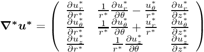$\mbox{\boldmath$ \nabla^* u^*$}$ is given by

$\mbox{\boldmath$ \nabla^* u^*$}= { \left(\begin{array}{ccc} \frac{\partial u^*_r}{\partial r^*}& \frac{1}{r^*}\frac{\partial u^*_r}{\partial\theta}-\frac{u^*_\theta}{r^*}& \frac{\partial u^*_r}{\partial z^*}\\ \frac{\partial u^*_\theta}{\partial r^*}& \frac{1}{r^*}\frac{\partial u^*_\theta}{\partial\theta}+\frac{u^*_r}{r^*}& \frac{\partial u^*_\theta}{\partial z^*}\\ \frac{\partial u^*_z}{\partial r^*}& \frac{1}{r^*}\frac{\partial u^*_z}{\partial\theta}& \frac{\partial u^*_z}{\partial z^*}\end{array}\right) }$

and $\mbox{\boldmath$\nabla^*\cdot u^*$}$ is equal to the trace of this matrix.

We non-dimensionalise the equations, using a problem specific reference length, ${\cal L}$ , and a timescale ${\cal T}=1/\omega$ , and use Young's modulus to non-dimensionalise the body force and the stress tensor:

$\mbox{\boldmath$ \tau^*$} = E \, \mbox{\boldmath$ \tau$}, \qquad r^* = {\cal L}\, r, \qquad z^* = {\cal L}\, z$

$\mbox{\boldmath$ u^*$} = {\cal L}\, \mbox{\boldmath$ u$}, \qquad \mbox{\boldmath$ F^*$} = \frac{E}{\rho \cal L} \, \mbox{\boldmath$ F$}, \qquad t^* = {\cal T}\, t.$

The non-dimensional form of the linear elasticity equations is then given by

$\mbox{\boldmath$ \nabla\cdot\tau$}+\mbox{\boldmath$ F$}=-\Omega^2\mbox{\boldmath$ u$}, \ \ \ \ \ \ \ \ \ \ (1)$

where $\mbox{\boldmath$ \nabla$}=(\frac{\partial}{\partial r},\frac{1}{r}\frac{\partial}{\partial\theta},\frac{\partial}{\partial z})$ ,

$\mbox{\boldmath$ \tau $}=\frac{1}{1+\nu}\left( \frac{\nu}{1-2\nu}(\mbox{\boldmath$\nabla\cdot u$})\textbf{I}+ \frac{1}{2}(\mbox{\boldmath$ \nabla u$}+\mbox{\boldmath$ \nabla u$}^{{\rm T}})\right), \ \ \ \ \ \ \ \ \ \ (2)$

and the non-dimensional parameter

$\Omega = {\cal L}\omega \sqrt{\frac{\rho}{E}}$

is the ratio of the elastic body's intrinsic timescale, ${\cal L} \sqrt{\frac{\rho}{E}}$ , to the problem-specific timescale, ${\cal T}=1/\omega$ , that we used to non-dimensionalise time. The boundary conditions are

$\mbox{\boldmath$ u$}=\mbox{\boldmath$ \hat{u}$}\,\,\textrm{on $ \partial D_d $},\quad \mbox{\boldmath$ \tau$}\cdot {\bf n} =\mbox{\boldmath$ \hat{\tau}$}\,\,\textrm{on $ \partial D_n $}.$

Given the assumed axisymmetry of the body we expand all quantities in a Fourier series in the azimuthal coordinate $\theta$ by writing,

$\mbox{\boldmath$ u$}(r,\theta ,z)=\sum_{n=-\infty}^{\infty}\mbox{\boldmath$ u$}^{(n)}(r,z){\rm e}^{{\rm i} n\theta},\quad \mbox{\boldmath$ F$} (r,\theta ,z)=\sum_{n=-\infty}^{\infty}\mbox{\boldmath$ F$}^{(n)}(r,z){\rm e}^{{\rm i} n\theta},\quad \mbox{\boldmath$ \tau$} (r,\theta ,z)=\sum_{n=-\infty}^{\infty}\mbox{\boldmath$ \tau$}^{(n)}(r,z){\rm e}^{{\rm i} n\theta} ,$

This decomposition allows us to remove the $\theta$ -dependence from the equations by writing $\frac{\partial\zeta}{\partial\theta}={\rm i}n\zeta$ , where $\zeta$ represents any physical parameter in the problem. Furthermore, since the governing equations are linear, we can solve for each Fourier component separately and simply specify the Fourier wavenumber 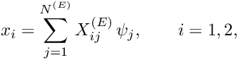as a parameter.

Implementation

Within oomph-lib, the non-dimensional version of the two-dimensional Fourier-decomposed equations (1) with the constitutive equations (2) are implemented in the TimeHarmonicFourierDecomposedLinearElasticityEquations equations class. Following our usual approach, discussed in the (Not-So-)Quick Guide, this equation class is then combined with a geometric finite element to form a fully-functional finite element. For instance, the combination of the TimeHarmonicFourierDecomposedLinearElasticityEquations class with the geometric finite element QElement<2,3> yields a nine-node quadrilateral element. As usual, the mapping between local and global (Eulerian) coordinates within an element is given by,

$x_i = \sum_{j=1}^{N^{(E)}} X^{(E)}_{ij} \, \psi_j, \qquad i=1,2,$

where the coordinates are enumerated as $x_1=r, \ x_2 = z$ . $N^{(E)}$ is the number of nodes in the element, $X^{(E)}_{ij}$ is the -th global (Eulerian) coordinate (enumerated as above) of the -th Node in the element, and the $\psi_j$ are the element's shape functions, defined in the geometric finite element.

We allow for the presence of damping by allowing the constitutive parameters and forcing frequency to be complex-valued. The three components of the displacement field therefore have real and imaginary parts and we store the six real-valued nodal unknowns in the order 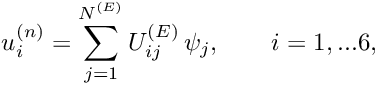$Re\{u_r^{(n)}\}, Re\{u_z^{(n)}\}, Re\{u_\theta^{(n)}\}, Im\{u_r^{(n)}\}, Im\{u_z^{(n)}\}, Im\{u_\theta^{(n)}\}$ and use the shape functions to interpolate the displacements as

$u_i^{(n)} = \sum_{j=1}^{N^{(E)}} U^{(E)}_{ij} \, \psi_j, \qquad i=1,...6,$

where $U^{(E)}_{ij}$ is the -th displacement component (enumerated as indicated above) at the -th Node in the element.

The test problem

The governing equations are fairly complicated and it is difficult to come up with non-trivial analytical solutions that could be used to validate the implementation. We therefore construct an analytical solution by postulating a displacement field and providing a body force that makes this a solution of the equations.

Specifically we consider the time-harmonic non-axisymmetric deformation of an annular elastic body that occupies the region 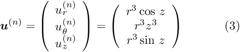$r_{\rm min}\leq r\leq r_{\rm max}, z_{\rm min}\leq z\leq z_{\rm max}, 0\leq\theta\leq 2\pi$ .

The displacement field

$\mbox{\boldmath$u$}^{(n)}= \left(\begin{array}{c}u_r^{(n)}\\u_\theta^{(n)}\\u_z^{(n)}\end{array}\right)= \left(\begin{array}{c}r^3\cos\, z\\r^3z^3\\r^3\sin\,z\end{array}\right) \ \ \ \ \ \ \ \ \ \ (3)$

is an exact solution of the governing equations if the body is subject to a body force

$\mbox{\boldmath$ F$}^{(n)}=\left(\begin{array}{c} -r(2{\rm i} nz^3\lambda+\cos\, z\{(8+3r)\lambda-(n^2-16+r(r-3))\mu+r^2 \Lambda^2\})\\ -r\{8z^3\mu-n^2z^3(\lambda+2\mu)+r^2(z^3\Lambda^2+6\mu z)+{\rm i} n\cos\, z((4+r)\lambda+(6+r)\mu)\}\\ r\sin\, z\{(n^2-9)\mu+4r(\lambda+\mu)+r^2(\lambda+2\mu-\Lambda^2)\}-3{\rm i} nr^2z^2(\lambda+\mu)\end{array}\right), \ \ \ \ \ \ \ \ \ \ (4)$

where $\lambda = \nu/((1+\nu)(1-2\nu))$ and $\mu = 1/(2(1+\nu))$ are the non-dimensional Lamé parameters (non-dimensionalised on ). The body is subject to a non-zero traction on all four boundaries; for example, on the inner boundary (where $r=r_{\rm min}$ ) the traction is

$\mbox{\boldmath$ \hat{\tau}$}^{(n)}_3= \mbox{\boldmath$ \tau$}^{(n)}(r_{\rm min},z)\cdot (-{\bf e}_r) = \left(\begin{array}{c} -6r_{\rm min}^2\mu\cos\, z-\lambda({\rm i} nr_{\rm min}^2z^3+r_{\rm min}^2(4+r_{\rm min})\cos\, z) \\ -\mu r_{\rm min}^2(2z^3+{\rm i} n\cos\, z) \\ -\mu r_{\rm min}^2\sin\, z(3-r_{\rm min}) \end{array}\right). \ \ \ \ \ \ \ \ \ \ (5)$

We choose to set this traction as a boundary condition, whilst pinning the displacements on the remaining boundaries where we impose a prescribed displacement according to (3).

Results

The figures below show plots of ${\rm Re}\{u_r^{(n)}\}, {\rm Re}\{u_z^{(n)}\}$ and ${\rm Re}\{u_\theta^{(n)}\}$ for a Fourier wavenumber of and geometric parameters $r_{\rm min}=0.1, r_{\rm max}=1.1, z_{\rm min}=0.3, z_{\rm max}=2.3$ . We set $\Omega^2=10+5{\rm i}$ , corresponding to an exponentially growing time-periodic forcing; $E=1+0.01{\rm i}$ , corresponding to a slightly dissipative material (see Comments ); and $\nu=0.3+0.05{\rm i}$ . The imaginary part of the solution is small (though not identically equal to zero) but it converges to zero under mesh refinement; see Exercises .

Computed (red) and exact (green) solution for real part of the radial displacement component.

Computed (red) and exact (green) solution for real part of the axial displacement component.

Computed (red) and exact (green) solution for real part of the azimuthal displacement component.

Global parameters and functions

As usual, we define all non-dimensional parameters in a namespace. In this namespace, we also define the (Fourier-decomposed) body force, the traction to be applied on boundary 3, and the exact solution. Note that, consistent with the enumeration of the unknowns, discussed above, the order of the components in the functions that specify the body force and the surface traction is $(r,z,\theta)$ .

//===start_of_namespace=================================================
/// Namespace for global parameters
//======================================================================
namespace Global_Parameters
{
 /// Define Poisson's ratio Nu
 std::complex<double> Nu(0.3,0.05);
 
 /// Define the non-dimensional Young's modulus
 std::complex<double> E(1.0,0.01);
 
 // Lame parameters
 std::complex<double> lambda = E*Nu/(1.0+Nu)/(1.0-2.0*Nu);
 std::complex<double> mu = E/2.0/(1.0+Nu);
 
 /// Define Fourier wavenumber
 int Fourier_wavenumber = 3;
 
 /// Define the non-dimensional square angular frequency of 
 /// time-harmonic motion
 std::complex<double> Omega_sq (10.0,5.0);
 
 /// Length of domain in r direction
 double Lr = 1.0;
 
 /// Length of domain in z-direction
 double Lz = 2.0;
 
 // Set up min & max (r,z) coordinates
 double rmin = 0.1;
 double zmin = 0.3;
 double rmax = rmin+Lr;
 double zmax = zmin+Lz;
 
 /// Define the imaginary unit
 const std::complex<double> I(0.0,1.0);
 
 /// The traction function at r=rmin: (t_r, t_z, t_theta)
 void boundary_traction(const Vector<double> &x,
                      const Vector<double> &n,
                      Vector<std::complex<double> > &result)
 {
  result[0] = -6.0*pow(x[0],2)*mu*cos(x[1])-
   lambda*(I*double(Fourier_wavenumber)*pow(x[0],2)*pow(x[1],3)+
           (4.0*pow(x[0],2)+pow(x[0],3))*cos(x[1]));
  result[1] = -mu*(3.0*pow(x[0],2)-pow(x[0],3))*sin(x[1]);
  result[2] = -mu*pow(x[0],2)*(2*pow(x[1],3)+I*double(Fourier_wavenumber)*
                               cos(x[1]));
 }
 
 
 /// The body force function; returns vector of complex doubles
 /// in the order (b_r, b_z, b_theta)
 void body_force(const Vector<double> &x,
                 Vector<std::complex<double> > &result)
 {
  result[0] = 
   x[0]*(-2.0*I*lambda*double(Fourier_wavenumber)*pow(x[1],3)-cos(x[1])*
         (lambda*(8.0+3.0*x[0])-
          mu*(pow(double(Fourier_wavenumber),2)
              -16.0+x[0]*(x[0]-3.0))+pow(x[0],2)*Omega_sq));
  result[1] = 
   x[0]*sin(x[1])*(mu*(pow(double(Fourier_wavenumber),2)-9.0)+
                   4.0*x[0]*(lambda+mu)+pow(x[0],2)*
                   (lambda+2.0*mu-Omega_sq))-
   3.0*I*double(Fourier_wavenumber)*pow(x[0],2)*pow(x[1],2)*(lambda+mu);
  result[2] = 
   -x[0]*(8.0*mu*pow(x[1],3)-pow(double(Fourier_wavenumber),2)*pow(x[1],3)*
          (lambda+2.0*mu)+pow(x[0],2)*(pow(x[1],3)*Omega_sq+6.0*mu*x[1])+
          I*cos(x[1])*double(Fourier_wavenumber)*
          (lambda*(4.0+x[0])+mu*(6.0+x[0])));
 }
 
 /// The exact solution in a flat-packed vector:
 // 0: u_r[real], 1: u_z[real],..., 5: u_theta[imag]
 void exact_solution(const Vector<double> &x,
                     Vector<double> &u)
 {
  u[0] = pow(x[0],3)*cos(x[1]);
  u[1] = pow(x[0],3)*sin(x[1]);
  u[2] = pow(x[0],3)*pow(x[1],3);
  u[3] = 0.0;
  u[4] = 0.0;
  u[5] = 0.0;
 }
 
} // end_of_namespace

The driver code

We start by setting the number of elements in each of the two coordinate directions before creating a DocInfo object to store the output directory.

//===start_of_main======================================================
/// Driver code 
//======================================================================
int main(int argc, char* argv[]) 
{
 // Number of elements in r-direction
 unsigned nr=5;
 
 // Number of elements in z-direction (for (approximately) square elements)
 unsigned nz=unsigned(double(nr)*Global_Parameters::Lz/Global_Parameters::Lr);
 
 // Set up doc info
 DocInfo doc_info;
 
 // Set output directory
 doc_info.set_directory("RESLT");

We build the problem using two-dimensional QTimeHarmonicFourierDecomposedLinearElasticityElements, solve using the Problem::newton_solve() function, and document the results.

 // Set up problem
 FourierDecomposedTimeHarmonicLinearElasticityProblem
  <QTimeHarmonicFourierDecomposedLinearElasticityElement<3> > 
  problem(nr,nz,Global_Parameters::rmin,Global_Parameters::rmax,
          Global_Parameters::zmin,Global_Parameters::zmax);
 
 // Solve
 problem.newton_solve();
 
 // Output the solution
 problem.doc_solution(doc_info);
  
} // end_of_main

The problem class

The Problem class is very simple. As in other problems with Neumann boundary conditions, we provide separate meshes for the "bulk" elements and the face elements that apply the traction boundary conditions. The latter are attached to the relevant faces of the bulk elements by the function assign_traction_elements().

//===start_of_problem_class=============================================
/// Class to validate time harmonic linear elasticity (Fourier 
/// decomposed)
//======================================================================
template<class ELEMENT>
class FourierDecomposedTimeHarmonicLinearElasticityProblem : public Problem
{
public:
 
 /// Constructor: Pass number of elements in r and z directions 
 /// and boundary locations
 FourierDecomposedTimeHarmonicLinearElasticityProblem(
 const unsigned &nr, const unsigned &nz,
 const double &rmin, const double& rmax,
 const double &zmin, const double& zmax);
 
 
 /// Update before solve is empty
 void actions_before_newton_solve() {}
 
 /// Update after solve is empty
 void actions_after_newton_solve() {}
 
 /// Doc the solution
 void doc_solution(DocInfo& doc_info);
 
private:
 
 /// Allocate traction elements on the bottom surface
 void assign_traction_elements();
 
 /// Pointer to the bulk mesh
 Mesh* Bulk_mesh_pt;
 
 /// Pointer to the mesh of traction elements
 Mesh* Surface_mesh_pt;
}; // end_of_problem_class

The problem constructor

We begin by building the meshes and pin the displacements on the appropriate boundaries. Recall that the order of the six real unknowns stored at the nodes is $\big(Re\{u_r^{(n)}\}, Re\{u_z^{(n)}\}, Re\{u_\theta^{(n)}\}, Im\{u_r^{(n)}\}, Im\{u_z^{(n)}\}, Im\{u_\theta^{(n)}\}\big).$

//===start_of_constructor=============================================
/// Problem constructor: Pass number of elements in coordinate
/// directions and size of domain.
//====================================================================
template<class ELEMENT>
FourierDecomposedTimeHarmonicLinearElasticityProblem<ELEMENT>::
FourierDecomposedTimeHarmonicLinearElasticityProblem
(const unsigned &nr, const unsigned &nz,
 const double &rmin, const double& rmax,
 const double &zmin, const double& zmax)
{
 //Now create the mesh
 Bulk_mesh_pt = new RectangularQuadMesh<ELEMENT>(nr,nz,rmin,rmax,zmin,zmax);
 
 //Create the surface mesh of traction elements
 Surface_mesh_pt=new Mesh;
 assign_traction_elements();
 
 // Set the boundary conditions for this problem: All nodes are
 // free by default -- just pin & set the ones that have Dirichlet 
 // conditions here
 
 // storage for nodal position
 Vector<double> x(2);
 
 // Storage for prescribed displacements
 Vector<double> u(6);
 
 // Now set displacements on boundaries 0 (z=zmin),
 //------------------------------------------------
 // 1 (r=rmax) and 2 (z=zmax)
 //--------------------------
 for (unsigned ibound=0;ibound<=2;ibound++)
  {
   unsigned num_nod=Bulk_mesh_pt->nboundary_node(ibound);
   for (unsigned inod=0;inod<num_nod;inod++) 
    {
     // Get pointer to node
     Node* nod_pt=Bulk_mesh_pt->boundary_node_pt(ibound,inod);
     
     // get r and z coordinates
     x[0]=nod_pt->x(0);
     x[1]=nod_pt->x(1);
     
     // Pinned in r, z and theta
     nod_pt->pin(0);nod_pt->pin(1);nod_pt->pin(2);
     nod_pt->pin(3);nod_pt->pin(4);nod_pt->pin(5);
     
     // Compute the value of the exact solution at the nodal point
     Vector<double> u(6);
     Global_Parameters::exact_solution(x,u);
     
     // Set the displacements
     nod_pt->set_value(0,u[0]);
     nod_pt->set_value(1,u[1]);
     nod_pt->set_value(2,u[2]);
     nod_pt->set_value(3,u[3]);
     nod_pt->set_value(4,u[4]);
     nod_pt->set_value(5,u[5]);
    }
  } // end_of_loop_over_boundary_nodes

Next we loop over the bulk mesh elements and assign the constitutive parameters, the body force, the Fourier wavenumber and the non-dimensional frequency to each element.

 // Complete the problem setup to make the elements fully functional
 
 // Loop over the elements
 unsigned n_el = Bulk_mesh_pt->nelement();
 for(unsigned e=0;e<n_el;e++)
  {
   // Cast to a bulk element
   ELEMENT *el_pt = dynamic_cast<ELEMENT*>(Bulk_mesh_pt->element_pt(e));
 
   // Set the body force
   el_pt->body_force_fct_pt() = &Global_Parameters::body_force;
 
   // Set the pointer to Poisson's ratio
   el_pt->nu_pt() = &Global_Parameters::Nu;
 
   // Set the pointer to Fourier wavenumber
   el_pt->fourier_wavenumber_pt() = &Global_Parameters::Fourier_wavenumber;
 
   // Set the pointer to non-dim Young's modulus
   el_pt->youngs_modulus_pt() = &Global_Parameters::E;
 
   // Set the pointer to square of the angular frequency
   el_pt->omega_sq_pt() = &Global_Parameters::Omega_sq;
 
  }// end loop over elements

We then loop over the traction elements and specify the applied traction.

 // Loop over the traction elements
 unsigned n_traction =  Surface_mesh_pt->nelement();
 for(unsigned e=0;e<n_traction;e++)
  {
   // Cast to a surface element
   TimeHarmonicFourierDecomposedLinearElasticityTractionElement<ELEMENT>*
    el_pt = 
    dynamic_cast<TimeHarmonicFourierDecomposedLinearElasticityTractionElement
    <ELEMENT>* >(Surface_mesh_pt->element_pt(e));
   
   // Set the applied traction
   el_pt->traction_fct_pt() = &Global_Parameters::boundary_traction;
   
  }// end loop over traction elements

The two sub-meshes are now added to the problem and a global mesh is constructed before the equation numbering scheme is set up, using the function assign_eqn_numbers().

 // Add the submeshes to the problem
 add_sub_mesh(Bulk_mesh_pt);
 add_sub_mesh(Surface_mesh_pt);
 
 // Now build the global mesh
 build_global_mesh();
 
 // Assign equation numbers
 cout << assign_eqn_numbers() << " equations assigned" << std::endl; 
 
} // end of constructor

The traction elements

We create the face elements that apply the traction to the boundary $r=r_{\rm min}$ .

//===start_of_traction===============================================
/// Make traction elements along the boundary r=rmin
//===================================================================
template<class ELEMENT>
void FourierDecomposedTimeHarmonicLinearElasticityProblem<ELEMENT>::
assign_traction_elements()
{
 unsigned bound, n_neigh;
 
 // How many bulk elements are next to boundary 3
 bound=3;
 n_neigh = Bulk_mesh_pt->nboundary_element(bound); 
 
 // Now loop over bulk elements and create the face elements
 for(unsigned n=0;n<n_neigh;n++)
  {
   // Create the face element
   FiniteElement *traction_element_pt 
    = new TimeHarmonicFourierDecomposedLinearElasticityTractionElement<ELEMENT>
    (Bulk_mesh_pt->boundary_element_pt(bound,n),
     Bulk_mesh_pt->face_index_at_boundary(bound,n));
 
   // Add to mesh
   Surface_mesh_pt->add_element_pt(traction_element_pt);
  }
 
} // end of assign_traction_elements

Post-processing

As expected, this member function documents the computed solution.

//==start_of_doc_solution=================================================
/// Doc the solution
//========================================================================
template<class ELEMENT>
void FourierDecomposedTimeHarmonicLinearElasticityProblem<ELEMENT>::
doc_solution(DocInfo& doc_info)
{ 
 ofstream some_file;
 char filename[100];
 
 // Number of plot points
 unsigned npts=5; 
 
 // Output solution 
 sprintf(filename,"%s/soln.dat",doc_info.directory().c_str());
 some_file.open(filename);
 Bulk_mesh_pt->output(some_file,npts);
 some_file.close();
 
 // Output exact solution 
 sprintf(filename,"%s/exact_soln.dat",doc_info.directory().c_str());
 some_file.open(filename);
 Bulk_mesh_pt->output_fct(some_file,npts,
                          Global_Parameters::exact_solution);
 some_file.close();
 
 // Doc error
 double error=0.0;
 double norm=0.0;
 sprintf(filename,"%s/error.dat",doc_info.directory().c_str());
 some_file.open(filename);
 Bulk_mesh_pt->compute_error(some_file,
                             Global_Parameters::exact_solution, 
                             error,norm);
 some_file.close();
 
 // Doc error norm:
 cout << "\nNorm of error:    " << sqrt(error) << std::endl; 
 cout << "Norm of solution: " << sqrt(norm) << std::endl << std::endl;
 cout << std::endl;
 
} // end_of_doc_solution   

Comments and Exercises

Comments

Given that we non-dimensionalised all stresses on Young's modulus it seems odd that we provide the option to specify a non-dimensional Young's modulus via the member function TimeHarmonicFourierDecomposedLinearElasticityEquations::youngs_modulus_pt(). The explanation for this is that this function specifies the ratio of the material's actual Young's modulus to the Young's modulus used in the non-dimensionalisation of the equations. The capability to specify such ratios is important in problems where the elastic body is made of multiple materials with different constitutive properties. If the body is made of a single, homogeneous material, the specification of the non-dimensional Young's modulus is not required – it defaults to 1.0. In the example considered above, the specification of the non-dimensional Young's modulus as $1 + 0.01 {\rm i}$
creates a small amount of damping in the material whose actual stiffness is still characterised by the (real-valued and dimensional) Young's modulus used to non-dimensionalise the equations.
Note that we also allow Poisson's ratio (whose specification is required) to be complex-valued. We are not aware of any meaningful physical interpretation of non-real Poisson ratios but provide this option because it appears to allow a better characterisation of some materials.

Exercises

Confirm that the specification of Poisson's ratio is required: What happens if you comment out its assignment in the problem constructor?
Confirm that the small imaginary part of the computed displacement field for the test problem goes to zero under mesh refinement.
Change the problem setup to the (less contrived) case where the deformation of the cylinder is driven by a time-periodic pressure load acting on the inside while its upper and lower ends are held at a fixed position. (You can cheat – there's another tutorial that shows you how to do it...).

Source files for this tutorial

The source files for this tutorial are located in the directory: demo_drivers/time_harmonic_fourier_decomposed_linear_elasticity/cylinder/
The driver code is: demo_drivers/time_harmonic_fourier_decomposed_linear_elasticity/cylinder/cylinder.cc

PDF file

A pdf version of this document is available.