Acknowledgement: This tutorial and the associated driver codes were developed jointly with David Nigro and Robert Harter (Thales Underwater Systems Ltd) with financial support from a KTA Secondment grant from University of Manchester's EPSRC-funded Knowledge Transfer Account.

In this document we discuss the solution of time-harmonic acoustic fluid-structure interaction problems in cylindrical polar coordinates, using a Fourier decomposition of the solution in the azimuthal direction. These equations are useful to solve problems involving axisymmetric elastic bodies.

We start by reviewing the relevant theory and then present the solution of a simple model problem – the sound radiation from an oscillating sphere that is coated with a compressible elastic layer.

This problem combines the problems discussed in the tutorials illustrating

the solution of the time-harmonic equations of linear elasticity in cylindrical polar coordinates

and

the Helmholtz equation in cylindrical polar coordinates

[Note that this tutorial is (obviously) very similar to its cartesian counterpart. The considerable overlap of material is deliberate to make both tutorials reasonably self-contained and explicit.]

Theory: Time-harmonic acoustic fluid-structure interaction problems in cylindrical polar coordinates

The figure below shows a sketch of a representative model problem: a sphere is immersed in an inviscid compressible fluid and performs a prescribed harmonic oscillation of radian frequency $\omega$ . The sphere is coated with a compressible elastic layer. We wish to compute the displacement field in the elastic coating (assumed to be described by the equations of time-harmonic linear elasticity) and the pressure distribution in the fluid (governed by the Helmholtz equation). The two sets of equations interact at the interface between fluid and solid: the fluid pressure exerts a traction onto the elastic layer, while the motion of the elastic layer drives the fluid motion via the non-penetration condition.

Sketch of the model problem: Forced oscillations of a sphere (black) deform an elastic coating layer (pink) which is surrounded by a compressible fluid.

The fluid model: the Helmholtz equation

We describe the behaviour of the fluid in terms of the displacement field, ${\bf d}^*(r^*,z^*,\varphi,t^*)$ , of the fluid particles, where and $\varphi$ are cylindrical polar coordinates. As usual, we use asterisks to distinguish dimensional quantities from their non-dimensional equivalents. The fluid is inviscid and compressible, with a bulk modulus , such that the acoustic pressure is given by $P^* = - B \ \nabla^{*} \cdot {\bf d}^*$ We assume that the fluid motion is irrotational and can be described by a displacement potential $\Phi^*$ , such that ${\bf d}^*= \nabla^* \Phi^*.$ We consider steady-state time-harmonic oscillations and write the displacement potential and the pressure as $\Phi^*(r^*,z^*,\varphi,t^*) = \mbox{Re} \{\phi^*(r^*,z^*,\varphi) \exp(-{\rm i} \omega t^*)\}$ and $P^*(r^*,z^*,\varphi,t^*) = \mbox{Re}\{p^*(r^*,z^*,\varphi) \exp(-{\rm i} \omega t^*)\}$ , respectively, where $\mbox{Re}\{\ldots \}$ denotes the real part. For small disturbances, the linearised Euler equation reveals that the time-harmonic pressure is related to the displacement potential via $p^* = \rho_{\rm f} \omega^2 \phi^*$ where $\rho_{\rm f}$ is the ambient fluid density. We non-dimensionalise all lengths on a problem-specific lengthscale ${\cal L}$ (e.g. the outer radius of the coating layer) such that $[r^*, z^*] = {\cal L} [r,z], \ {\bf d}^* = {\cal L} {\bf d}$ and $\phi^* = {\cal L}^2 \phi$ .

We then decompose $\phi$ into its Fourier components by writing

${\phi}(r,\varphi,z) = \sum_{N=-\infty}^{\infty} \phi_N(r,z) \exp({\rm i} N \varphi).$

Since the governing equations are linear we can compute each Fourier component $\phi_N(r,z)$ individually by solving

$\nabla^2 {\phi_{N}}(r,z) + \left(k^2-\frac{N^2}{r^2}\right) \phi_N(r,z) = 0, \ \ \ \ \ \ \ \ \ \ \ \ (1)$

where the square of the non-dimensional wavenumber,

$k^2 = \frac{\rho_{\rm f} (\omega {\cal L})^2}{B},$

represents the ratio of the typical inertial fluid pressure induced by the wall oscillation to the ‘stiffness’ of the fluid.

The solid model: the time harmonic equations of linear elasticity

We model the coating layer as a linearly elastic solid, described in terms of a displacement field ${\bf U}^*(r^*,z^*,\varphi,t^*)$ , with stress tensor

$\mbox{\boldmath$ \tau^*$}=\frac{E}{1+\nu}\left( \frac{\nu}{1-2\nu}(\mbox{\boldmath$\nabla^*\cdot U^*$})\textbf{I}+ \frac{1}{2}(\mbox{\boldmath$ \nabla^* U^*$}+ \mbox{\boldmath$ \nabla^* U^*$}^{{\rm T}})\right),$

where and $\nu$ are the material's Young's modulus and Poisson's ratio, respectively.

As before, we assume a time-harmonic solution with frequency $\omega$ so that ${\bf U}^*(r^*,z^*,\varphi,t^*) = {\rm Re} \{ {\bf u}^*(r^*,z^*,\varphi) \exp(-{\rm i}\omega t^*)\}$ . We non-dimensionalise the displacements on ${\cal L}$ and the stress on Young's modulus, , so that ${\bf u}^* = {\cal L} {\bf u}$ and $\mbox{\boldmath$ \tau^*$} = E \mbox{\boldmath$ \tau$}$ . The deformation of the elastic coating is then governed by the time-harmonic Navier-Lame equations

$\mbox{\boldmath$ \nabla\cdot\tau$}+\Omega^2\mbox{\boldmath$ u$} = {\bf 0} \ \ \ \ \ \ \ \ \ \ (2)$

where

$\mbox{\boldmath$ \tau $}=\frac{1}{1+\nu}\left( \frac{\nu}{1-2\nu}(\mbox{\boldmath$\nabla\cdot u$})\textbf{I}+ \frac{1}{2}(\mbox{\boldmath$ \nabla u$}+\mbox{\boldmath$ \nabla u$}^{{\rm T}})\right) \ \ \ \ \ \ \ \ \ \ (3)$

is the non-dimensional stress tensor. The (square of the) non-dimensional wavenumber

$\Omega^2 = \frac{\rho_{\rm s} (\omega {\cal L})^2}{E},$

where $\rho_{\rm s}$ is the solid density, represents the ratio of the typical inertial solid pressure induced by the wall oscillation to the stiffness of the elastic coating. We note that for a ‘light’ coating we have $\Omega \ll 1$ .

We then decompose ${\bf u}$ into its Fourier components by writing

${\bf u}(r,\varphi,z) = \sum_{N=-\infty}^{\infty} {\bf u}_N(r,z) \exp({\rm i} N \varphi).$

This decomposition allows us to remove the $\theta$ -dependence from the equations by writing $\partial (.)/\partial\theta={\rm i} N (.)$ . Since the governing equations are linear, we can solve for each Fourier component separately and specify the Fourier wavenumber as a parameter.

Boundary conditions

The inner surface of the elastic coating, $\partial D_{\rm s}$ , is subject to the prescribed displacement imposed by the oscillating cylinder. For instance, if the inner cylinder performs spherically symmetric oscillations of non-dimensional amplitude $\epsilon$ , we have

$\mbox{\bf u}_0 = \epsilon \, \mbox{\bf e}_{r_{\rm sphere}} \mbox{\ \ \ \ \ on $\partial D_{\rm s}$}, \ \ \ \ \ \ \ \ \ \ \ \ \ \ \ \ \ \ \ \ \ \ (4)$

where

$\mbox{\bf e}_{r_{\rm sphere}} = \frac{r}{\sqrt{r^2+z^2}} {\bf e}_r + \frac{z}{\sqrt{r^2+z^2}} {\bf e}_z$

is the unit vector in the (spherically!) radial direction, while the other Fourier components remain zero, $\mbox{\bf u}_j = {\bf 0}$ for $j=\pm 1, \pm 2, ...$ The fluid-loaded surface of the elastic coating, $\partial D_{\rm f}$ , is subject to the fluid pressure. The non-dimensional traction exerted by the fluid onto the solid (on the solid stress scale) is therefore given by

${\bf t}^{\rm [solid]} = \mbox{\boldmath$ \tau $}^{\rm [solid]} \cdot {\bf n} = - \phi \ Q \ {\bf n} \mbox{\ \ \ \ \ on $\partial D_{\rm f}$}, \ \ \ \ \ \ \ \ \ \ \ \ \ \ \ \ \ \ \ \ \ \ (5)$

where the ${\bf n} = n_r {\bf e}_r + n_z {\bf e}_z$ is the outer unit normal on the solid boundary $\partial D_{\rm f}$ and

$Q=\frac{\rho_{\rm f}({\cal L}\omega)^2}{E}$

is the final non-dimensional parameter in the problem. It represents the ratio of the typical inertial fluid pressure induced by the wall oscillation to the stiffness of the elastic coating. The parameter therefore provides a measure of the strength of the fluid-structure interaction (FSI) in the sense that for $Q \to 0$ the elastic coating does not ‘feel’ the presence of the fluid.

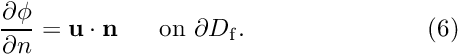The fluid is forced by the normal displacement of the solid. Imposing the non-penetration condition $({\bf d} - {\bf u}) \cdot {\bf n} = 0$ on $\partial D_{\rm f}$ yields a Neumann condition for the displacement potential,

$\frac{\partial \phi}{\partial n} = {\bf u} \cdot {\bf n} \mbox{\ \ \ \ \ on $\partial D_{\rm f}$}. \ \ \ \ \ \ \ \ \ \ \ \ \ \ \ \ \ \ \ \ \ \ (6)$

Finally, the displacement potential for the fluid must satisfy the Sommerfeld radiation condition

$\lim_{r_{\rm sphere} \to \infty} r_{\rm sphere} \left( \frac{\partial \phi}{\partial r_{\rm sphere} } - {\rm i} k \phi \right) = 0, \ \ \ \ \ \ \ \ \ \ \ \ \ \ \ \ \ \ \ \ \ \ (7)$

where $r_{\rm sphere} = \sqrt{(r^2+z^2)}$ is the (spherical) radius. The Sommerfeld radiation condition ensures that the oscillating sphere does not generate any incoming waves.

Equations (5), (6) and (7) apply for each Fourier component of the solution.

Implementation

The implementation of the coupled problem follows the usual procedure for multi-domain problems in oomph-lib. We discretise the constituent single-physics problems using the existing single-physics elements, here oomph-lib's

Helmholtz elements

and

time-harmonic linear elasticity elements

for the discretisation of the PDEs (1) and (2), respectively. The displacement boundary condition (4) on the inner surface of the elastic coating is imposed as usual by pinning the relevant degrees of freedom, exactly as in a single-physics solid mechanics problem. Similarly, the Sommerfeld radiation condition (7) on the outer boundary of the fluid domain can be imposed by any of the methods available for the solution of the single-physics Helmholtz equation, such as a Dirichlet-to-Neumann mapping.

The boundary conditions (5) and (6) at the fluid-solid interface are traction boundary conditions for the solid, and Neumann boundary conditions for the Helmholtz equation, respectively. In a single-physics problem we would impose such boundary conditions by attaching suitable FaceElements to the appropriate boundaries of the "bulk" elements, as shown in the sketch below: TimeHarmonicFourierDecomposedLinearElasticityTractionElement could be used to impose a (given) traction, ${\bf t}_0$ , onto the solid; FourierDecomposedHelmholtzFluxElements could be used to impose a (given) normal derivative, , on the displacement potential. Both ${\bf t}_0$ and would usually be specified in a user-defined namespace and accessed via function pointers as indicated in the right half of the sketch.

Sketch illustrating the imposition of flux and traction boundary conditions in single-physics problems. The continuous problems are shown on the left; the discretised ones on the right.

In the coupled problem, illustrated in the left half of the next sketch, the traction acting on the solid becomes a function of the displacement potential via the boundary condition (5), while the normal derivative of the displacement potential is given in terms of the solid displacement via equation (6). Note that corresponding points on the FSI boundary $\partial D_{\rm f}$ are identified by matching values of the boundary coordinate $\zeta$ which is assumed to be consistent between the two domains.

The implementation of this interaction in the discretised problem is illustrated in the right half of the sketch: We replace the single-physics FourierDecomposedHelmholtzFluxElements by FourierDecomposedHelmholtzFluxFromNormalDisplacementBCElements, and the TimeHarmonicFourierDecomposedLinearElasticityTractionElements by FourierDecomposedTimeHarmonicLinElastLoadedByHelmholtzPressureBCElements. (Yes, we like to be verbose...). Both of these FaceElements are derived from the ElementWithExternalElement base class and can therefore store a pointer to an "external" element that provides the information required to impose the appropriate boundary condition. Thus, the FourierDecomposedHelmholtzFluxFromNormalDisplacementBCElements store pointers to the "adjacent" time-harmonic linear elasticity elements (from which they obtain the boundary displacement required for the imposition of (6)), while the FourierDecomposedTimeHarmonicLinElastLoadedByHelmholtzPressureBCElements store pointers to the "adjacent" Helmholtz elements that provide the value of the displacement potential required for the evaluation of (5).

Sketch illustrating the imposition of flux and traction boundary conditions in the coupled multi-physics problem. The continuous problems are shown on the left; the discretised ones on the right.

The identification of the "adjacent" bulk elements can be performed using the Multi_domain_functions::setup_bulk_elements_adjacent_to_face_mesh(...) helper function. We note that, as suggested by the sketch above, this function does not require to the two adjacent meshes to have a consistent discretisation – the identification of adjacent elements is based entirely on the (assumed to be consistent) boundary coordinate $\zeta$ in the two meshes. We refer to another tutorial for a discussion of how to set up (or change) the parametrisation of mesh boundaries by boundary coordinates.

Results

The animation below shows the deformation of the elastic coating if a non-spherically symmetric displacement

$\mbox{\bf u} = \epsilon \, \mbox{\bf e}_{r_{\rm sphere}} \cos (M\theta) \mbox{\ \ \ \ \ on $\partial D_{\rm s}$}, \ \ \ \ \ \ \ \ \ \ \ \ \ \ \ \ \ \ \ \ \ \ (8)$

(for ) where $\theta$ is the zenith angle, is imposed on the inner boundary of the coating $\partial D_{\rm s}$ .

Animation showing the time-harmonic oscillation of the elastic coating. (The pink region in the background shows the undeformed configuration.)

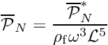Here is a plot of the corresponding pressure field:

Plot of the displacement potential (a measure of the fluid pressure). The elevation in the carpet plot indicates the real part; the colour contours represent the imaginary part.

Finally, we provide some validation of the computational results by comparing the non-dimensional time-average radiated power

$\overline{\cal P }_N = \frac{\overline{\cal P }^*_N}{\rho_{\rm f} \omega^3 {\cal L}^5}$

(see Appendix: The time-averaged radiated power for details) against the analytical solution for spherically symmetric forcing ( ) for the parameter values , $\rho_{\rm solid}/\rho_{\rm fluid} =1.0$ , $\nu =0.3$ and a non-dimensional coating thickness of

Radiated power as function of the FSI parameter Q for a spherically-symmetrically oscillating coating. Markers: computed results; continuous line: analytical result.

Real part of the fluid displacement potential (a measure of the fluid pressure) for Q=10. Shaded: computed; spheres: exact.

Imaginary part of the fluid displacement potential (a measure of the fluid pressure) for Q=10. Shaded: computed; spheres: exact.

Real part of the radial solid displacement for Q=10. Shaded: computed; spheres: exact.

Imaginary part of the radial solid displacement for Q=10. Shaded: computed; spheres: exact.

Real part of the axial solid displacement for Q=10. Shaded: computed; spheres: exact.

Imaginary part of the axial solid displacement for Q=10. Shaded: computed; spheres: exact.

The numerical solution

The global namespace

As usual we define the problem parameters in a namespace. (Recall that we allow the constitutive parameters to be complex-valued.)

//=======start_of_namespace==========================================
/// Global variables
//===================================================================
namespace Global_Parameters
{
 
 /// Square of wavenumber for the Helmholtz equation
 double K_squared=10.0;
 
 /// Radius of outer boundary of Helmholtz domain
 double Outer_radius=2.0; 
 
 /// FSI parameter
 double Q=10.0;
 
 /// Non-dim thickness of elastic coating
 double H_coating=0.2; 
 
 /// Define azimuthal Fourier wavenumber
 int Fourier_wavenumber=0;
   
 /// Poisson's ratio Nu
 std::complex<double> Nu(std::complex<double>(0.3,0.0));

We wish to perform parameter studies in which we vary the FSI parameter . To make this physically meaningful, we interpret $Q =(\rho_{\rm f}({\cal L}\omega)^2)/E$ as a measure of the stiffness of the elastic coating (so that an increase in corresponds to a reduction in the layer's elastic modulus ). In that case, the frequency parameter $\Omega^2 = (\rho_{\rm s} (\omega {\cal L})^2)/E$ in the time-harmonic linear elasticity equations becomes a dependent parameter and is given in terms of the density ratio $\rho_{\rm solid}/\rho_{\rm fluid}$ and by $\Omega^2 = (\rho_{\rm solid}/\rho_{\rm fluid}) Q$ . We therefore provide a helper function to update the dependent parameter following any change in the independent parameters.

 
 /// Non-dim square of frequency for solid -- dependent variable!
 std::complex<double>  Omega_sq(std::complex<double>(100.0,0.0));
 
 /// Density ratio: solid to fluid
 double Density_ratio=1.0; 
 
 /// Function to update dependent parameter values
 void update_parameter_values()
 {
  Omega_sq=Density_ratio*Q;
 }

We force the system by imposing a prescribed displacement on the inner surface of the elastic coating and allow this to vary in the "zenith"-direction with wavenumber :

 
 /// Wavenumber "zenith"-variation of imposed displacement of coating
 /// on inner boundary 
 unsigned M=4; 
 
 /// Displacement field on inner boundary of solid
 void solid_boundary_displacement(const Vector<double>& x,
                                  Vector<std::complex<double> >& u)
 {
  Vector<double> normal(2);
  double norm=sqrt(x[0]*x[0]+x[1]*x[1]);
  double theta=atan2(x[1],x[0]);
  normal[0]=x[0]/norm;
  normal[1]=x[1]/norm;
 
  u[0]=complex<double>(normal[0]*cos(double(M)*theta),0.0);
  u[1]=complex<double>(normal[1]*cos(double(M)*theta),0.0);
 }

Finally, we specify the output directory and a multiplier for the number of elements in the meshes to aid mesh convergence studies.

 
 /// Output directory
 string Directory="RESLT";
 
 /// Multiplier for number of elements
 unsigned El_multiplier=1;
 
} //end_of_namespace

The driver code

The driver code is very straightforward. We parse the command line to determine the parameters for the parameter study and build the problem object, using nine-noded quadrilateral elements for the solution of the time-harmonic elasticity and Helmholtz equations.

//=======start_of_main==================================================
/// Driver for coated sphere loaded by lineared fluid loading
//======================================================================
int main(int argc, char **argv)
{
 
 // Store command line arguments
 CommandLineArgs::setup(argc,argv);
 
 // Define possible command line arguments and parse the ones that
 // were actually specified
 
 // Output directory
 CommandLineArgs::specify_command_line_flag("--dir",
                                            &Global_Parameters::Directory);
 
 // Parameter for the Helmholtz equation
 CommandLineArgs::specify_command_line_flag("--k_squared",
                                            &Global_Parameters::K_squared);
 
 // Initial value of Q 
 CommandLineArgs::specify_command_line_flag("--q_initial", 
                                            &Global_Parameters::Q);
 
 // Number of steps in parameter study
 unsigned nstep=2;
 CommandLineArgs::specify_command_line_flag("--nstep",&nstep);
 
 // Increment in FSI parameter in parameter study
 double q_increment=5.0;
 CommandLineArgs::specify_command_line_flag("--q_increment",&q_increment);
 
 
 // Wavenumber "zenith"-variation of imposed displacement of coating
 // on inner boundary 
 CommandLineArgs::specify_command_line_flag("--M",
                                            &Global_Parameters::M);
 
 // Multiplier for number of elements
 CommandLineArgs::specify_command_line_flag("--el_multiplier",
                                            &Global_Parameters::El_multiplier);
 
 // Parse command line
 CommandLineArgs::parse_and_assign(); 
 
 // Doc what has actually been specified on the command line
 CommandLineArgs::doc_specified_flags();
 
 // Update dependent parameters values
 Global_Parameters::update_parameter_values();
 
 // Set up doc info
 DocInfo doc_info;
 
 // Set output directory
 doc_info.set_directory(Global_Parameters::Directory);
 
 // Set up the problem
 CoatedSphereProblem<QTimeHarmonicFourierDecomposedLinearElasticityElement<3>,
                     QFourierDecomposedHelmholtzElement<3> > problem;

We then solve the problem for various values of , updating the dependent variables after every increment.

 
 //Parameter incrementation
 for(unsigned i=0;i<nstep;i++)
  {
   // Solve the problem with Newton's method
   problem.newton_solve();
 
   // Doc solution
   problem.doc_solution(doc_info);
 
   // Increment FSI parameter
   Global_Parameters::Q+=q_increment;
   Global_Parameters::update_parameter_values();
  }
 
} //end_of_main

The problem class

The Problem class is templated by the types of the "bulk" elements used to discretise the Fourier-decomposed time-harmonic linear elasticity and Helmholtz equations, respectively. It contains the usual member functions to attach FaceElements to the bulk meshes in order to apply the various Neumann boundary conditions. We note that the costly recomputation of the $\gamma-$ integral in the Dirichlet-to-Neumann mapping before the Newton convergence check (implemented in actions_before_newton_convergence_check()) can be avoided by declaring the problem to be linear; see the discussion in the Helmholtz tutorial and Comments.

//=============start_of_problem_class===================================
/// Coated sphere FSI
//====================================================================== 
template<class ELASTICITY_ELEMENT, class HELMHOLTZ_ELEMENT>
class CoatedSphereProblem : public Problem
{
 
public:
 
 /// Constructor:
 CoatedSphereProblem();
 
 /// Update function (empty)
 void actions_before_newton_solve(){}
 
 /// Update function (empty)
 void actions_after_newton_solve() {}
 
 /// Recompute gamma integral before checking Newton residuals
 void actions_before_newton_convergence_check()
  {
   Helmholtz_DtN_mesh_pt->setup_gamma();
  }
  
 /// Doc the solution
 void doc_solution(DocInfo& doc_info);
 
private:
 
 /// Create FSI traction elements
 void create_fsi_traction_elements();
 
 /// Create Helmholtz FSI flux elements
 void create_helmholtz_fsi_flux_elements(); 
 
 /// Setup interaction
 void setup_interaction();
 
 /// Create DtN elements on outer boundary
 void create_helmholtz_DtN_elements();

The private member data includes storage for the various meshes and objects that are used for outputting the results.

 
 /// Pointer to solid mesh
 TwoDAnnularMesh<ELASTICITY_ELEMENT>* Solid_mesh_pt;
 
 /// Pointer to mesh of FSI traction elements
 Mesh* FSI_traction_mesh_pt;
 
 /// Pointer to Helmholtz mesh
 TwoDAnnularMesh<HELMHOLTZ_ELEMENT>* Helmholtz_mesh_pt;
 
 /// Pointer to mesh of Helmholtz FSI flux elements
 Mesh* Helmholtz_fsi_flux_mesh_pt;
 
 /// Pointer to mesh containing the DtN elements
 FourierDecomposedHelmholtzDtNMesh<HELMHOLTZ_ELEMENT>* Helmholtz_DtN_mesh_pt;
 
 /// Trace file
 ofstream Trace_file;
 
};// end_of_problem_class

The problem constructor

We start by building the meshes for the elasticity and Helmholtz equations. Both domains are half annular regions, so the annular mesh (which is built from a rectangular QuadMesh) is not periodic but only occupies 180 degrees. The mesh also needs to be rotated by 90 degrees to align its ends with the axis:

//===========start_of_constructor======================================= 
/// Constructor: 
//====================================================================== 
template<class ELASTICITY_ELEMENT, class HELMHOLTZ_ELEMENT>
CoatedSphereProblem<ELASTICITY_ELEMENT, HELMHOLTZ_ELEMENT>::
CoatedSphereProblem() 
{
 
 // Parameters for meshes
 bool periodic=false;
 double azimuthal_fraction_of_coating=0.5;
 double phi=0.5*MathematicalConstants::Pi;

The solid mesh occupies the region between and where is the thickness of the elastic coating:

 
 // Solid mesh
 //-----------
 // Number of elements in azimuthal direction
 unsigned ntheta_solid=10*Global_Parameters::El_multiplier;
 
 // Number of elements in radial direction 
 unsigned nr_solid=3*Global_Parameters::El_multiplier;
 
 // Innermost radius for solid mesh
 double a=1.0-Global_Parameters::H_coating;
 
 // Build solid mesh
 Solid_mesh_pt = new 
  TwoDAnnularMesh<ELASTICITY_ELEMENT>(periodic,azimuthal_fraction_of_coating,
                                      ntheta_solid,nr_solid,a,
                                      Global_Parameters::H_coating,phi);

The Helmholtz mesh occupies the region between and $r=R_{\rm outer}$ where $R_{\rm outer}$ is the outer radius of the computational domain where we will apply the Sommerfeld radiation condition. Note that the two meshes are not matching – both meshes have 3 element layers in the radial direction but 10 and 11 in the azimuthal direction, respectively. This is done mainly to illustrate our claim that the multi-domain setup functions can operate with non-matching meshes.

 
 
 // Helmholtz mesh
 //---------------
 
 // Number of elements in azimuthal direction in Helmholtz mesh
 unsigned ntheta_helmholtz=11*Global_Parameters::El_multiplier;
 
 // Number of elements in radial direction in Helmholtz mesh
 unsigned nr_helmholtz=3*Global_Parameters::El_multiplier;
 
 // Innermost radius of Helmholtz mesh
 a=1.0;
 
 // Thickness of Helmholtz mesh
 double h_thick_helmholtz=Global_Parameters::Outer_radius-a;
 
 // Build mesh
 Helmholtz_mesh_pt = new TwoDAnnularMesh<HELMHOLTZ_ELEMENT>
  (periodic,azimuthal_fraction_of_coating,
   ntheta_helmholtz,nr_helmholtz,a,h_thick_helmholtz,phi);

Next we create the mesh that will store the FaceElements that will apply the Sommerfeld radiation condition, using the specified number of Fourier terms in the Dirichlet-to-Neumann mapping; see the Helmholtz tutorial for details.

 
 
 // Create mesh for DtN elements on outer boundary
 unsigned nfourier=20;
 Helmholtz_DtN_mesh_pt=
  new FourierDecomposedHelmholtzDtNMesh<HELMHOLTZ_ELEMENT>(
   Global_Parameters::Outer_radius,nfourier);

Next we pass the problem parameters to the bulk elements. The elasticity elements require a pointer to Poisson's ratio, $\nu$ , the azimuthal (Fourier) wavenumber , and the frequency parameter $\Omega^2$ :

 
 // Complete the solid problem setup to make the elements fully functional
 unsigned nel=Solid_mesh_pt->nelement();
 for (unsigned e=0;e<nel;e++)
  {     
   // Cast to a bulk element
   ELASTICITY_ELEMENT* el_pt=dynamic_cast<ELASTICITY_ELEMENT*>(
    Solid_mesh_pt->element_pt(e));
 
   // Set the pointer to Fourier wavenumber
   el_pt->fourier_wavenumber_pt() = &Global_Parameters::Fourier_wavenumber;
   
   // Set the pointer to Poisson's ratio
   el_pt->nu_pt() = &Global_Parameters::Nu;
      
   // Set the pointer to square of the angular frequency
   el_pt->omega_sq_pt() = &Global_Parameters::Omega_sq;
  }

The Helmholtz elements need a pointer to the (square of the) wavenumber, and the azimuthal (Fourier) wavenumber :

 
 // Complete the build of all Helmholtz elements so they are fully functional
 unsigned n_element = Helmholtz_mesh_pt->nelement();
 for(unsigned i=0;i<n_element;i++)
  {
   // Upcast from GeneralsedElement to the present element
   HELMHOLTZ_ELEMENT *el_pt = dynamic_cast<HELMHOLTZ_ELEMENT*>(
    Helmholtz_mesh_pt->element_pt(i));
   
   //Set the k_squared pointer
   el_pt->k_squared_pt()=&Global_Parameters::K_squared;
   
   // Set pointer to Fourier wave number
   el_pt->fourier_wavenumber_pt()=&Global_Parameters::Fourier_wavenumber;
  }

It is always a good idea to check the enumeration of the mesh boundaries to facilitate the application of boundary conditions:

 
 // Output meshes and their boundaries so far so we can double 
 // check the boundary enumeration
 Solid_mesh_pt->output("solid_mesh.dat");
 Helmholtz_mesh_pt->output("helmholtz_mesh.dat");
 Solid_mesh_pt->output_boundaries("solid_mesh_boundary.dat");
 Helmholtz_mesh_pt->output_boundaries("helmholtz_mesh_boundary.dat");

Next we create the meshes containing the various FaceElements used to apply to the FSI traction boundary condition (5), the FSI flux boundary condition (6) for the Helmholtz equation, and the Sommerfeld radiation condition (7), respectively, using helper functions discussed below.

 
 // Create FaceElement meshes for boundary conditions
 //--------------------------------------------------
 
 // Construct the fsi traction element mesh
 FSI_traction_mesh_pt=new Mesh;
 create_fsi_traction_elements();
 
 // Construct the Helmholtz fsi flux element mesh
 Helmholtz_fsi_flux_mesh_pt=new Mesh;
 create_helmholtz_fsi_flux_elements();
 
 // Create DtN elements
 create_helmholtz_DtN_elements();

We add the various sub-meshes to the problem and build the global mesh

 
 
 // Combine sub meshes
 //-------------------
 add_sub_mesh(Solid_mesh_pt);
 add_sub_mesh(FSI_traction_mesh_pt);
 add_sub_mesh(Helmholtz_mesh_pt);
 add_sub_mesh(Helmholtz_fsi_flux_mesh_pt);
 add_sub_mesh(Helmholtz_DtN_mesh_pt); 
 
 // Build the Problem's global mesh from its various sub-meshes
 build_global_mesh();

The solid displacements are prescribed on the inner boundary (boundary 0) of the solid mesh so we pin all six values (representing the real and imaginary parts of the displacements in the and $\varphi-$ directions, respectively) and assign the boundary values using the function Global_Parameters::solid_boundary_displacement(...). (The enumeration of the unknowns in the Fourier-decomposed equations time-harmonic linear elasticity is discussed in another tutorial.)

 
 
 // Solid boundary conditions:
 //---------------------------
 
 // Pin the solid inner boundary (boundary 0) in all directions
 unsigned b=0;
 unsigned n_node = Solid_mesh_pt->nboundary_node(b);
 
 Vector<std::complex<double> > u(2);
 Vector<double> x(2);
 
 //Loop over the nodes to pin and assign boundary displacements on 
 //solid boundary
 for(unsigned i=0;i<n_node;i++)
  {
   Node* nod_pt=Solid_mesh_pt->boundary_node_pt(b,i);
   nod_pt->pin(0);
   nod_pt->pin(1);
   nod_pt->pin(2);
   nod_pt->pin(3);
   nod_pt->pin(4);
   nod_pt->pin(5);
 
   // Assign prescribed displacements
   x[0]=nod_pt->x(0);
   x[1]=nod_pt->x(1);
   Global_Parameters::solid_boundary_displacement(x,u);
 
   // Real part of radial displacement
   nod_pt->set_value(0,u[0].real());
   // Real part of axial displacement
   nod_pt->set_value(1,u[1].real());
   // Real part of azimuthal displacement
   nod_pt->set_value(2,0.0);
   // Imag part of radial displacement
   nod_pt->set_value(3,u[0].imag());
   // Imag part of axial displacement
   nod_pt->set_value(4,u[1].imag());
   // Imag part of azimuthal displacement
   nod_pt->set_value(5,0.0);
  }

The radial and azimuthal displacements have to vanish on the symmetry boundary (boundaries 1 and 3):

 
 // Vertical Symmetry boundary (r=0 and z<0)
 {
  unsigned ibound=1;
  {
   unsigned num_nod= Solid_mesh_pt->nboundary_node(ibound);
   for (unsigned inod=0;inod<num_nod;inod++)
    {
     // Get pointer to node
     Node* nod_pt=Solid_mesh_pt->boundary_node_pt(ibound,inod);
     
     // Pin radial displacement (u_0 (real) and u_3 (imag))
     nod_pt->pin(0);
     nod_pt->set_value(0,0.0);
     nod_pt->pin(3);
     nod_pt->set_value(3,0.0);
     
     // Pin azimuthal displacement (u_2 (real) and u_5 (imag))
     nod_pt->pin(2);
     nod_pt->set_value(2,0.0);
     nod_pt->pin(5);
     nod_pt->set_value(5,0.0);
    }
  }
 }
 
 
 // Vertical Symmetry boundary (r=0 and z>0)
 {
  unsigned ibound=3;
  {
   unsigned num_nod= Solid_mesh_pt->nboundary_node(ibound);
   for (unsigned inod=0;inod<num_nod;inod++)
    {
     // Get pointer to node
     Node* nod_pt=Solid_mesh_pt->boundary_node_pt(ibound,inod);
     
     // Pin radial displacement (u_0 (real) and u_3 (imag))
     nod_pt->pin(0);
     nod_pt->set_value(0,0.0);
     nod_pt->pin(3);
     nod_pt->set_value(3,0.0);
     
     // Pin azimuthal displacement (u_2 (real) and u_5 (imag))
     nod_pt->pin(2);
     nod_pt->set_value(2,0.0);
     nod_pt->pin(5);
     nod_pt->set_value(5,0.0);
    }
  }
 } // done sym bc

Finally, we set up the fluid-structure interaction, assign the equation numbers and open a trace file to record the radiated power as a function of the FSI parameter .

 
 // Setup fluid-structure interaction
 //----------------------------------
 setup_interaction();
 
 // Open trace file
 char filename[100];
 sprintf(filename,"%s/trace.dat",Global_Parameters::Directory.c_str());
 Trace_file.open(filename);
  
 // Setup equation numbering scheme
 cout <<"Number of equations: " << assign_eqn_numbers() << std::endl; 
 
}//end_of_constructor

Creating the FSI traction elements (and the FSI flux and DtN elements)

The function create_fsi_traction_elements() creates the FaceElements required to apply the FSI traction boundary condition (5) on the outer boundary (boundary 2) of the solid mesh:

//============start_of_create_fsi_traction_elements======================
/// Create fsi traction elements 
//=======================================================================
template<class ELASTICITY_ELEMENT, class HELMHOLTZ_ELEMENT>
void CoatedSphereProblem<ELASTICITY_ELEMENT,HELMHOLTZ_ELEMENT>::
create_fsi_traction_elements()
{
 // We're on boundary 2 of the solid mesh
 unsigned b=2;
 
 // How many bulk elements are adjacent to boundary b?
 unsigned n_element = Solid_mesh_pt->nboundary_element(b);
 
 // Loop over the bulk elements adjacent to boundary b
 for(unsigned e=0;e<n_element;e++)
  {
   // Get pointer to the bulk element that is adjacent to boundary b
   ELASTICITY_ELEMENT* bulk_elem_pt = dynamic_cast<ELASTICITY_ELEMENT*>(
    Solid_mesh_pt->boundary_element_pt(b,e));
   
   //Find the index of the face of element e along boundary b
   int face_index = Solid_mesh_pt->face_index_at_boundary(b,e);
   
   // Create element
   FourierDecomposedTimeHarmonicLinElastLoadedByHelmholtzPressureBCElement
    <ELASTICITY_ELEMENT,HELMHOLTZ_ELEMENT>* el_pt=
    new FourierDecomposedTimeHarmonicLinElastLoadedByHelmholtzPressureBCElement
    <ELASTICITY_ELEMENT,HELMHOLTZ_ELEMENT>(bulk_elem_pt,
                                           face_index);   
   // Add to mesh
   FSI_traction_mesh_pt->add_element_pt(el_pt);

To function properly, the elements need to know the number of the bulk mesh boundary they are attached to (this allows them to determine the boundary coordinate $\zeta$ required to set up the fluid-structure interaction; see Implementation ), and the FSI parameter .

   
   // Associate element with bulk boundary (to allow it to access
   // the boundary coordinates in the bulk mesh)
   el_pt->set_boundary_number_in_bulk_mesh(b); 
   
   // Set FSI parameter
   el_pt->q_pt()=&Global_Parameters::Q;
  }
 
} // end_of_create_fsi_traction_elements

[Note: We omit the listings of the functions create_helmholtz_fsi_flux_elements() and create_helmholtz_DtN_elements() which create the FaceElements required to apply the FSI flux boundary condition (6) on the inner boundary (boundary 0), and the Sommerfeld radiation condition (7) on the outer boundary (boundary 2) of the Helmholtz mesh because they are very similar. Feel free to inspect the
source code.]

Setting up the fluid-structure interaction

The setup of the fluid-structure interaction requires the identification of the "bulk" Helmholtz elements that are adjacent to (the Gauss points of) the FaceElements that impose the FSI traction boundary condition (5), in terms of the displacement potential $\phi$ computed by these "bulk" elements. This can be done using the helper function Multi_domain_functions::setup_bulk_elements_adjacent_to_face_mesh(...) which is templated by the type of the "bulk" element and its spatial dimension, and takes as arguments:

a pointer to the Problem,
the boundary ID of the FSI boundary in the "bulk" mesh,
a pointer to that mesh,
a pointer to the mesh of FaceElements.

Nearly a one-liner (if you ignore the optional output of the boundary coordinate which allows us to check that the FSI boundaries of the fluid and solid domains have been parametrised consistently).

//=====================start_of_setup_interaction======================
/// Setup interaction between two fields
//========================================================================
template<class ELASTICITY_ELEMENT, class HELMHOLTZ_ELEMENT>
void CoatedSphereProblem<ELASTICITY_ELEMENT,HELMHOLTZ_ELEMENT>::
setup_interaction()
{
 
 // Setup Helmholtz "pressure" load on traction elements
 unsigned boundary_in_helmholtz_mesh=0;
 
 // Doc boundary coordinate for Helmholtz
 ofstream the_file;
 the_file.open("boundary_coordinate_hh.dat");
 Helmholtz_mesh_pt->Mesh::template doc_boundary_coordinates<HELMHOLTZ_ELEMENT>
  (boundary_in_helmholtz_mesh, the_file);
 the_file.close();
 
 // Setup interaction
  Multi_domain_functions::setup_bulk_elements_adjacent_to_face_mesh
  <HELMHOLTZ_ELEMENT,2>
  (this,boundary_in_helmholtz_mesh,Helmholtz_mesh_pt,FSI_traction_mesh_pt);

Exactly the same method can be used for the identification of the "bulk" elasticity elements that are adjacent to (the Gauss points of) the FaceElements that impose the FSI flux boundary condition (6), using the displacement ${\bf u}$ computed by these "bulk" elements:

 
 // Setup Helmholtz flux from normal displacement interaction
 unsigned boundary_in_solid_mesh=2;
 
 // Doc boundary coordinate for solid mesh
 the_file.open("boundary_coordinate_solid.dat");
 Solid_mesh_pt->Mesh::template doc_boundary_coordinates<ELASTICITY_ELEMENT>
  (boundary_in_solid_mesh, the_file);
 the_file.close();
 
 // Setup interaction
 Multi_domain_functions::setup_bulk_elements_adjacent_to_face_mesh
  <ELASTICITY_ELEMENT,2>(
   this,boundary_in_solid_mesh,Solid_mesh_pt,Helmholtz_fsi_flux_mesh_pt);
 
}// end_of_setup_interaction

Post-processing

The post-processing function doc_solution(...) computes and outputs the total radiated power, and plots the computed solutions (real and imaginary parts) for all fields.

//==============start_of_doc_solution===============================
/// Doc the solution
//==================================================================
template<class ELASTICITY_ELEMENT, class HELMHOLTZ_ELEMENT>
void CoatedSphereProblem<ELASTICITY_ELEMENT,HELMHOLTZ_ELEMENT>::
doc_solution(DocInfo& doc_info)
{
 
 // Doc parameters
 oomph_info << "Writing result for step " << doc_info.number() 
            << ". Parameters: "<< std::endl;
 oomph_info << "Fourier mode number : N = "
            << Global_Parameters::Fourier_wavenumber << std::endl;
 oomph_info << "FSI parameter : Q = " << Global_Parameters::Q << std::endl;
 oomph_info << "Fluid outer radius : R = " << Global_Parameters::Outer_radius
            << std::endl;
 oomph_info << "Fluid wavenumber : k^2 = " << Global_Parameters::K_squared
            << std::endl;
 oomph_info << "Solid wavenumber : Omega_sq = " << Global_Parameters::Omega_sq 
            << std::endl << std::endl; 
 
 
 ofstream some_file,some_file2;
 char filename[100];
 
 // Number of plot points
 unsigned n_plot=5; 
 
 // Compute/output the radiated power
 //----------------------------------
 sprintf(filename,"%s/power%i.dat",doc_info.directory().c_str(),
         doc_info.number());
 some_file.open(filename);
 
 // Accumulate contribution from elements
 double power=0.0;
 unsigned nn_element=Helmholtz_DtN_mesh_pt->nelement(); 
 for(unsigned e=0;e<nn_element;e++)
  {
   FourierDecomposedHelmholtzBCElementBase<HELMHOLTZ_ELEMENT> *el_pt = 
    dynamic_cast<FourierDecomposedHelmholtzBCElementBase<HELMHOLTZ_ELEMENT>*>(
     Helmholtz_DtN_mesh_pt->element_pt(e)); 
   power += el_pt->global_power_contribution(some_file);
  }
 some_file.close();
 oomph_info << "Radiated power: " << power << std::endl;
 
 // Output displacement field
 //--------------------------
 sprintf(filename,"%s/elast_soln%i.dat",doc_info.directory().c_str(),
         doc_info.number());
 some_file.open(filename);
 Solid_mesh_pt->output(some_file,n_plot);
 some_file.close();
 
 // Output Helmholtz
 //-----------------
 sprintf(filename,"%s/helmholtz_soln%i.dat",doc_info.directory().c_str(),
         doc_info.number());
 some_file.open(filename);
 Helmholtz_mesh_pt->output(some_file,n_plot);
 some_file.close();
 
 
 // Output fsi traction elements
 //----------------------------- 
 sprintf(filename,"%s/fsi_traction_soln%i.dat",doc_info.directory().c_str(),
         doc_info.number());
 some_file.open(filename);
 FSI_traction_mesh_pt->output(some_file,n_plot);
 some_file.close();
 
 
 // Output Helmholtz fsi flux elements
 //----------------------------------- 
 sprintf(filename,"%s/fsi_flux_bc_soln%i.dat",doc_info.directory().c_str(),
         doc_info.number());
 some_file.open(filename);
 Helmholtz_fsi_flux_mesh_pt->output(some_file,n_plot);
 some_file.close();
 
 // Write trace file
 Trace_file << Global_Parameters::Q << " " 
            << Global_Parameters::K_squared << " "
            << Global_Parameters::Density_ratio << " "
            << Global_Parameters::Omega_sq.real() << " "
            << power << " " 
            << std::endl;
   
 // Bump up counter
 doc_info.number()++;
 
} //end_of_doc_solution

Comments and Exercises

Comments

The application of the Sommerfeld radiation condition via a Dirichlet-to-Neumann mapping is discussed in detail in another tutorial. We explain there that, because the $\gamma$ integral depends on the solution, it must be recomputed whenever the unknowns are updated during the Newton iteration. This is best done by adding a call to FourierDecomposedHelmholtzDtNMesh::setup_gamma() to Problem::actions_before_newton_convergence_check() as done in the driver code listed above. However, if Helmholtz's equation is solved in isolation (or within a coupled, but linear problem as in the present case ), the Newton method is guaranteed to converge in one iteration. In such cases the unnecessary recomputation of $\gamma$ after the one-and-only Newton iteration can be suppressed by setting Problem::Problem_is_nonlinear to false – in that case, oomph-lib's Newton solver skips the convergence check in the Newton iteration and simply accepts the solution obtained after one linear solve.
You may have noticed that, unlike the tutorial for the cartesian counterpart of the model problem considered here, we neither demonstrate how to apply the Sommerfeld radiation condition by approximate/absorbing boundary conditions (ABCs), nor do we demonstrate the use of spatial adaptivity. This is because the relevant elements have not (yet!) been written (Any volunteers?). If you wish to enable spatial adaptivity we suggest using an unstructured adaptive mesh, using the methodology demonstrated in another tutorial.

Exercises

As shown in the Appendix: The time-averaged radiated power, the time-averaged radiated power $\overline{\cal P}$ depends on the derivatives of the displacement potential $\phi$ . This implies that the value for $\overline{\cal P}$ computed from the finite-element solution for $\phi$ is not as accurate as the displacement potential itself. Computing $\overline{\cal P}$ to a certain tolerance (e.g. to "graphical accuracy" as in the plot shown above) therefore tends to require meshes that are much finer than would be required if we were only interested in $\phi$ itself.

Investigate the accuracy of the computational predictions for $\overline{\cal P}$ by:
- increasing the spatial resolution e.g. by using the command line flag --el_multiplier which controls the number of elements in the mesh.
- reducing the outer radius of the computational domain, using the command line flag --outer_radius, say.
- varying the element type, from the bi-linear QFourierDecomposedHelmholtzElement<2> to the bi-cubic QFourierDecomposedHelmholtzElement<4>, say.
Which of these approaches gives you the "most accuracy" for a given number of degrees of freedom?

Appendix: The time-averaged radiated power

This appendix provides a brief summary of the computation (and non-dimensionalisation) of the time-averaged power $\overline{\cal P }^*$ radiated across the closed surface $\partial V$ (with outer unit normal ${\bf n}$ ) of a fluid volume . In dimensional terms, $\overline{\cal P }^*$ is given by

$\overline{\cal P }^* = \oint_{\partial V} I^* dA^*, \ \ \ \ \ \ \ \ \ \ \ (9)$

where the intensity

$I^* = \frac{1}{{\cal T}} \int_0^{\cal T} {\bf U}^* \cdot P^* {\bf n} \ dt^*$

depends on the fluid velocity ${\bf U}^* = \partial {\bf d}^*/\partial t^* = \partial/\partial t^* (\nabla^* \Phi^*)$ and the pressure $P^* = \rho_{\rm f} \omega^2 \Phi^*$ . The time average is taken over the period of the oscillation, 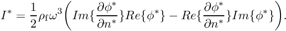${\cal T} = 2\pi/\omega.$ Using our time-periodic ansatz for the fluid displacement potential, $\Phi^* = Re\{ \phi^* \exp(-{\rm i}\omega t^*) \}$ , the intensity can be re-written as

$I^* = \frac{1}{2} \rho_{\rm f} \omega^3 \bigg( Im \{\frac{\partial \phi^*}{\partial n^*} \} Re\{\phi^* \} - Re \{\frac{\partial \phi^*}{\partial n^*} \} Im\{\phi^* \} \bigg).$

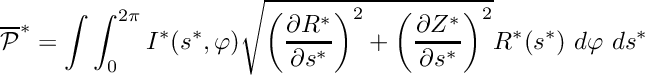Next we express the surface integral in (9) in cylindrical polar coordinates. Assuming the (axisymmetric) boundary of the fluid domain is parametrised (in the plane) as and , where is some curve parameter (e.g. the arclength), we have

$\overline{\cal P }^* = \int \int_0^{2\pi} I^*(s^*,\varphi) \sqrt{ \left(\frac{\partial R^*}{\partial s^*}\right)^2 + \left(\frac{\partial Z^*}{\partial s^*}\right)^2 } R^*(s^*) \ d\varphi \ ds^*$

The power associated with the th azimuthal Fourier mode, $\phi^*_N(r^*,z^*) \exp({\rm i}N \varphi)$ , is then given by

$\overline{\cal P }^*_N = \pi \rho_{\rm f} \omega^3 \int \bigg( Im \{\frac{\partial \phi_N^*}{\partial n^*} \} Re\{\phi_N^* \} - Re \{\frac{\partial \phi_N^*}{\partial n^*} \} Im\{\phi_N^* \} \bigg) \sqrt{ \left(\frac{\partial R^*}{\partial s^*}\right)^2 + \left(\frac{\partial Z^*}{\partial s^*}\right)^2 } R^*(s^*) \ ds^*.$

Non-dimensionalising all lengths on ${\cal L}$ and the displacement potential on ${\cal L}^2$ then yields the following expression for the non-dimensional time-averaged radiated power

$\overline{\cal P }_N = \frac{\overline{\cal P }^*_N}{\rho_{\rm f} \omega^3 {\cal L}^5} = \pi \int \bigg( Im \{\frac{\partial \phi_N}{\partial n} \} Re\{\phi_N \} - Re \{\frac{\partial \phi_N}{\partial n} \} Im\{\phi_N \} \bigg) \sqrt{ \left(\frac{\partial R}{\partial s}\right)^2 + \left(\frac{\partial Z}{\partial s}\right)^2 } R(s) \ ds.$

This quantity is computed by oomph-lib on an element-by-element basis, using the function FourierDecomposedHelmholtzBCElementBase::global_power_contribution(...).

The computation is most easily validated by comparing against analytical results in which the displacement potential is expressed in spherical polar coordinates $(r_{\rm sphere}^*, \theta, \varphi)$ where $r_{\rm sphere}^* = \sqrt{r^{*2} + z^{*2}}$ and $\theta$ is the zenith angle which varies from $\theta=0$ at the "North pole" to 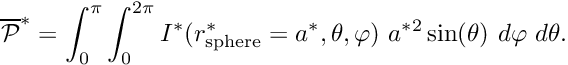$\theta=\pi$ at the "South pole". If we evaluate the surface integral in (9) on a spherical surface of dimensional radius , the dimensional time-averaged radiated power is

$\overline{\cal P }^* = \int_0^\pi \int_0^{2\pi} I^*(r_{\rm sphere}^*=a^*, \theta,\varphi)\ a^{*2} \sin(\theta) \ d\varphi \ d\theta.$

The power associated with th azimuthal Fourier mode, $\phi^*_N(r^*,z^*) \exp({\rm i}N \varphi)$ , is then given by

$\overline{\cal P }^*_N = \pi a^{*2} \rho_{\rm f} \omega^3 \int_0^\pi \left.\bigg( Im \{\frac{\partial \phi_N^*}{\partial n^*} \} Re\{\phi_N^* \} - Re \{\frac{\partial \phi_N^*}{\partial n^*} \} Im\{\phi_N^* \} \bigg)\right|_{r_{\rm sphere}^*=a^*} \sin(\theta) \ d\theta,$

where $\partial / \partial n^* = \partial / \partial r_{\rm sphere}^*$ . The non-dimensional time-averaged power, evaluated on a sphere of non-dimensional radius $a = a^*/{\cal L}$ is then given by

$\overline{\cal P }_N = \frac{\overline{\cal P }^*_N}{\rho_{\rm f} \omega^3 {\cal L}^5} = \pi a^2 \int_0^\pi \left. \bigg( Im \{\frac{\partial \phi_N}{\partial n} \} Re\{\phi_N \} - Re \{\frac{\partial \phi_N}{\partial n} \} Im\{\phi_N \} \bigg)\right|_{r_{\rm sphere}=a} \sin(\theta) \ d\theta,$

where $\partial / \partial n = \partial / \partial r_{\rm sphere}$ .

The derivation of the analytical expression for $\overline{\cal P }_N$ against which we validated our computational results were performed with maple, using the script demo_drivers/interaction/fourier_decomposed_acoustic_fsi/exact.map .

Source files for this tutorial

The source files for this tutorial are located in the directory: demo_drivers/interaction/fourier_decomposed_acoustic_fsi/
The driver code is: demo_drivers/interaction/fourier_decomposed_acoustic_fsi/fourier_decomposed_acoustic_fsi.cc

PDF file

A pdf version of this document is available.